
A n
2
RNA SECONDARY STRUCTURE PREDICTION ALGORITHM
Markus E. Nebel and Anika Scheid
∗
Department of Computer Science, University of Kaiserslautern, P.O. Box 3049, D-67653 Kaiserslautern, Germany
Keywords:
RNA folding, RNA secondary structure, Computational prediction, Probabilistic modeling, Stochastic
context-free grammars, Statistical sampling, Inside-outside calculation, Heuristic approximation.
Abstract:
Several state-of-the-art tools for predicting RNA secondary structures have worst-case time and space require-
ments of O(n
3
) and O(n
2
) for sequence length n, limiting their applicability for practical purposes. Accord-
ingly, biologists are interested in getting results faster, where a moderate loss of accuracy would willingly be
tolerated. For this reason, we propose a novel algorithm for structure prediction that reduces the time com-
plexity by a linear factor to O(n
2
), while still being able to produce high quality results. Basically, our method
relies on a probabilistic sampling approach based on an appropriate stochastic context-free grammar (SCFG):
using a well-known or a newly introduced sampling strategy it generates a random set of candidate structures
(from the ensemble of all feasible foldings) according to a “noisy” distribution (obtained by heuristically ap-
proximating the inside-outside values) for a given sequence, such that finally a corresponding prediction can
be efficiently derived. Sampling can easily be parallelized. Furthermore, it can be done in-place, i.e. only
the best (most probable) candidate structure generated so far needs to be stored and finally communicated.
Together, this allows to efficiently handle increased sample sizes necessary to achieve competitive prediction
accuracy in connection with the noisy distribution.
1 INTRODUCTION
Over the past years, several new approaches towards
the prediction of RNA secondary structures from a
single sequence have been invented which are based
on generating statistically representative and repro-
ducible samples of the entire ensemble of feasible
structures for the given sequence. For example, the
popular Sfold software (Ding and Lawrence, 2003;
Ding et al., 2004) employs a sampling extension
of the partition function (PF) approach (McCaskill,
1990) to produce statistically representative subsets
of the Boltzmann-weighted ensemble. More recently,
a corresponding probabilistic method has been stud-
ied (Nebel and Scheid, 2011) which actually sam-
ples the possible foldings from a distribution implied
by a sophisticated stochastic context-free grammar
(SCFG).
Notably, both sampling methods can be extended
for predicting secondary structures in O(n
3
) time and
with O(n
2
) space requirements, respectively. These
worst-case complexities are actually identical to those
of modern state-of-the-art tools for computational
∗
Corresponding author. The research of this author has
been supported by the Carl-Zeiss-Stiftung.
structure prediction from a single sequence, for in-
stance the commonly used minimum free energy
(MFE) based Mfold (Zuker, 1989; Zuker, 2003) and
Vienna RNA (Hofacker et al., 1994; Hofacker, 2003)
packages or the popular SCFG based Pfold soft-
ware (Knudsen and Hein, 1999; Knudsen and Hein,
2003). Furthermore, applications to structure predic-
tion showed that neither of the two competing sam-
pling approaches (SCFG and PF based method) gen-
erally outperforms the other and consequently, it is
not obvious which one should rather be preferred in
practice. This somehow contradicts the fact that the
best physics-based prediction methods still generally
perform significantly better than the best probabilis-
tic approaches. In principle, only if the computa-
tional effort of one particular variant could be im-
proved without significant losses in quality (that is if
one of them required considerably less time than the
others while it sacrificed only little predictive accu-
racy), then the corresponding method would be un-
doubtably the number one choice for practical appli-
cations, indeed outperforming all other modern com-
putational tools for predicting the secondary structure
of RNA sequences. This, by the way, due to the of-
ten quite large sizes of native RNA molecules consid-
66
E. Nebel M. and Scheid A..
A n2 RNA SECONDARY STRUCTURE PREDICTION ALGORITHM.
DOI: 10.5220/0003764600660075
In Proceedings of the International Conference on Bioinformatics Models, Methods and Algorithms (BIOINFORMATICS-2012), pages 66-75
ISBN: 978-989-8425-90-4
Copyright
c
2012 SCITEPRESS (Science and Technology Publications, Lda.)

ered in practice, meets exactly the demands imposed
by biologists on computational prediction procedures:
rather getting moderately less accurate (but still good
quality) results in less time than needing significantly
more time for obtaining results that are expectedly not
considerably more accurate.
Note that recently, there already have been sev-
eral practical heuristic speedups (Wexler et al., 2007;
Backofen et al., 2011). Particularly, the approach
of (Wexler et al., 2007) for folding single RNA se-
quences manages to speed up the standard dynamic
programming algorithms without sacrificing the opti-
mality of the results, yielding an expected time com-
plexity of O(n
2
· ψ(n)), where ψ(n) is shown to be
constant on average under standard polymer fold-
ing models; in (Backofen et al., 2011), it is shown
how to reduce those average-case time and space
complexities in the sparse case. Furthermore, the
practical technique from (Frid and Gusfield, 2010)
achieves an improved worst-case time complexity of
O(n
3
/log(n)), and with the (MFE and SCFG based)
algorithms from (Akutsu, 1999), a slight worst-case
speedup of O(n
3
· log(log(n))
1/2
/log(n)
1/2
) time can
be reached (whose practicality is unlikely and un-
established).
In this article, we present a new way to reduce the
worst-case time complexity of SCFG based statisti-
cal sampling by a linear factor, making it possible
to predict for instance the most probable (MP) struc-
ture among all feasible foldings for a given input se-
quence of length n (in direct analogy to conventional
structure prediction via SCFGs) with only O(n
2
) time
and space requirements. This complexity improve-
ment is basically realized by employing an appropri-
ate heuristic instead of the corresponding exact algo-
rithm for preprocessing the input sequence, i.e. for
deriving a “noisy” distribution (induced by heuristic
approximations of the corresponding inside and out-
side probabilities) on the entire structure ensemble
for the input sequence. From this distribution candi-
date structures can be efficiently sampled.
2
Moreover,
we will consider two different sampling strategies: (a
slight modification of) the widely known sampling
procedure from (Ding and Lawrence, 2003; Nebel
and Scheid, 2011) which basically generates a ran-
dom structure from outside to inside, and a novel al-
ternative strategy that obeys to contrary principles and
employs a reverse course of action (from inside to out-
side) but manages to take more advantage of the ap-
2
With purposive proof-of-concept implementations (in
Wolfram Mathematica 7.0), for instance the overall prepro-
cessing time for E.coli tRNA
Ala
(of length n = 76) could be
reduced from 49.0 (traditional cubic algorithm) to only 3.7
(new quadratic strategy) seconds.
proximative preprocessing.
As we will see, even building on our new heuris-
tic preprocessing step, both sampling strategies can
be applied to obtain MP structure predictions of re-
spectable accuracy. In principle, for sufficiently large
sample sizes we obtain a similar high predictive accu-
racy as in the case of exact calculations
3
. The seem-
ingly sole pitfall is that due to the noisy ensemble dis-
tribution resulting from approximative computations,
the resulting samples are no longer guaranteed to pri-
marily contain rather likely structures (with respect to
the exact distribution of feasible foldings for a given
input sequence), such that we usually have to gen-
erate more candidate structures (i.e., consider larger
sample sizes) in oder to ensure reproducible structure
predictions. However, this is quite unproblematic in
practice: firstly, we can generate the candidate struc-
tures in-place (only the so far most probable structure
needs to be stored), such that large sample sizes give
no rise to memory consumption and secondly, gen-
erating samples can easily be parallelized on modern
multi-core architectures or grids.
2 PRELIMINARIES
In the sequel, given an RNA molecule r consisting of
n nucleotides, we denote the corresponding sequence
fragment from position i to position j, 1 ≤ i ≤ j ≤ n,
by R
i, j
= r
i
r
i+1
...r
j−1
r
j
. Accordingly, S
i, j
denotes a
feasible secondary structure on R
i, j
.
2.1 Sampling based on SCFG Model
Briefly, probabilistic sampling based on a suitable
SCFG G
s
with sets I
G
s
and R
G
s
of intermediate sym-
bols and productions, respectively, and axiom S ∈ I
G
s
(that models the class of all feasible secondary struc-
tures) has two basic steps: In the first step (prepro-
cessing), all inside probabilities
α
X
(i, j) := Pr(X ⇒
∗
lm
r
i
...r
j
) (1)
and all outside probabilities
β
X
(i, j) := Pr(S ⇒
∗
lm
r
1
...r
i−1
X r
j+1
...r
n
) (2)
for a sequence r of size n, X ∈ I
G
s
and 1 ≤ i, j ≤ n, are
computed. According to (Nebel and Scheid, 2011),
this can be done with a special variant of an Earley-
style parser (such that the considered grammar does
not need to be in Chomsky normal form (CNF)),
3
For E.coli tRNA
Ala
, we for instance observed the same
sensitivity and specificity values of 1.0 and 0.91, respec-
tively, with a particular application of our heuristic method
and the corresponding exact variant.
A n2 RNA SECONDARY STRUCTURE PREDICTION ALGORITHM
67

where the grammar parameters (trained beforehand
on a suitable RNA structure database) are splitted into
a set of transition probabilities Pr
0
tr
(rule) for rule ∈
R
G
s
and two sets of emission probabilities Pr
1
em
(·) for
the 4 unpaired bases and the 16 possible base pairings.
For any such SCFG G
s
, there results O(n
3
) time com-
plexity and O(n
2
) memory requirement for this pre-
processing step. Note that in this work, we will use
the sophisticated grammar from (Nebel and Scheid,
2011) which has been parameterized to impose two
relevant restrictions on the class of all feasible struc-
tures, namely a minimum length of min
HL
for hairpin
loops and a minimum number of min
hel
consecutive
base pairs for helices.
The second step takes the form of a recursive sam-
pling algorithm to randomly draw a complete sec-
ondary structure by consecutively sampling substruc-
tures (defined by base pairs and unpaired bases). No-
tably, different sampling strategies may be employed
for realizing this step; two contrary variants that will
be considered within this work are described in detail
in Section 4. In general, for any sampling decision
(for example choice of a new base pair), the strategy
considers the respective set of all possible choices that
might actually be formed on the currently considered
fragment of the input sequence. Any of these sets con-
tains exactly the mutually and exclusive cases as de-
fined by the alternative productions (of a particular in-
termediate symbol) of the underlying grammar. The
corresponding random choice is then drawn accord-
ing to the resulting conditional sampling distribution
(for the considered sequence fragment). This means
that the respective sampling distributions are defined
by the inside and outside values derived in step one
(providing information on the distribution of all pos-
sible choices according to the actual input sequence)
and the grammar parameters (transition probabilities).
Since every of the before mentioned conditional
distributions needed for randomly drawing one of the
respective possible choices can be derived in linear
time (during the sampling process), any valid
4
base
pair can be sampled in time O(n). Thus, since any
structure of size n can have at most b
n−min
HL
2
c base
pairs, a random candidate structure for the given input
sequence can be generated in O(n
2
) time.
Thus, one straightforward approach for improving
the performance of the overall sampling algorithm in
the worst-case is to reduce the O(n
3
) time complex-
4
One may for example consider only the 6 different
most stable canonical pairs as valid ones (like usually done
in physics-based approaches due to missing thermodynam-
ics parameters for non-canonical pairs). However, we de-
cided to drop this restriction, considering all possible non-
crossing base pairings to be valid.
ity required for the preprocessing step at least to the
quadratic time of the sampling strategy. To us, this
means we might be able to save a significant amount
of time by replacing the exact inside-outside calcula-
tions with a corresponding heuristic method yielding
only approximative inside-outside values for a given
input sequence. To see if this might actually be suc-
cessful, we next want to determine to which extend
the inside and outside probabilities react to different
types and degrees of disturbances in order the get evi-
dence if it could actually be possible to find an appro-
priate heuristic.
2.2 Disturbance Types and Levels
We decided to disturb the exact inside and outside
probabilities for a given input sequence r of length n
in the following ways: For each X ∈ I
G
s
and 1 ≤ i, j ≤
n, redefine the corresponding inside value according
to
α
X
(i, j) := max(min(α
X
(i, j) + α
err
,1),0), (3)
where α
err
is randomly chosen from the following in-
terval or set:
[−max
ErrPerc
α
A
(i, j),+max
ErrPerc
α
A
(i, j)] or
{−fix
ErrPerc
α
A
(i, j),+fix
ErrPerc
α
A
(i, j)}
(relative errors), with max
ErrPerc
,fix
ErrPerc
∈ (0, 1]
defining percentages, or else,
[−max
ErrVal
,+max
ErrVal
] or {−fix
ErrVal
,+fix
ErrVal
}
(absolute errors), with max
ErrVal
,fix
ErrVal
∈ (0,1] be-
ing fixed values. Random errors on all outside values
β
X
(i, j), X ∈ I
G
s
and 1 ≤ i, j ≤ n, can be generated in
the same way.
The needed conditional sampling distributions (as
considered by a particular strategy) are then derived
from the exact grammar parameters and the disturbed
inside-outside probabilities for the input sequence.
This might create the need to (slightly) modify a par-
ticularly employed sampling strategy for being capa-
ble of dealing with these skewed distributions, as we
will see in Section 4.1.
2.3 Analysis of Disturbance Influence
To get a first impression on the influence of distur-
bances (in the ensemble distribution for a given input
sequence) on the quality of generated sample sets, we
opted for the potentially most intuitive application in
this context, namely probability profiling for unpaired
bases within particular loop types (see, e.g., (Ding and
Lawrence, 2003)). In principle, for each nucleotide
position i, 1 ≤ i ≤ n, of a given sequence of length
BIOINFORMATICS 2012 - International Conference on Bioinformatics Models, Methods and Algorithms
68

0
10
20
30
40
50
60
70
0.0
0.2
0.4
0.6
0.8
1.0
Nucleotide Position
Probability
Hplot
Figure 1: Hairpin loop profile and MP prediction obtained
for E.coli tRNA
Ala
. All results have been derived from sam-
ples of size 1,000, generated with min
hel
= 2 and min
HL
=
3. Errors were produced with max
ErrPerc
= 0.99 (thick
gray lines) and fix
ErrPerc
= 0.99 (thick dotted darker gray
lines).The profiles also display the respective exact results
(thin black lines) and the native folding of E.coli tRNA
Ala
(black points).
0
10
20
30
40
50
60
70
0.0
0.2
0.4
0.6
0.8
1.0
Nucleotide Position
Probability
Hplot
Figure 2: Sampling results for E.coli tRNA
Ala
correspond-
ing to those presented in Figure 1, where max
ErrVal
= 10
−9
(thick gray lines) and fix
ErrVal
= 10
−9
(thick dotted darker
gray lines) have been chosen for generating the distur-
bances.
n, one computes the probabilities that i is an unpaired
base within a specific loop type. These probabilities
are given by the observed frequencies in a represen-
tative statistical sample of the complete ensemble (of
all possible secondary structures) for the given input
sequence.
Furthermore, in order to investigate to what ex-
tend the accuracy of predicted foldings changes when
different dimensions of relative disturbances are in-
corporated into the needed sampling probabilities, we
will additionally derive the most probable (MP) struc-
ture in the generated samples, respectively, as predic-
tion. Note that for our examinations, we will exem-
plarily consider a well-known trusted tRNA structure,
Escherichia coli tRNA
Ala
, since this molecule folds
into the typical cloverleaf structure, making it very
easy to judge the accuracy of the resulting profiles and
predictions.
Figure 1 indicates that even in the case of large
relative errors, the sampled structures still exhibit
the typical cloverleaf structure of tRNAs, especially
for the extenuated disturbance variant according to
max
ErrPerc
which seems to have practically no effect
on the resulting sampling quality and prediction ac-
curacy. However, Figure 2 perfectly demonstrates
that if the disturbances have been created by gener-
ating absolute errors on all inside values, then – even
for rather small values – the resulting samples (and
corresponding predictions as well) seem to be use-
less. Nevertheless, it seems reasonable to believe that
the inside and outside probabilities do not necessarily
have to be computed in the exact way, but it may prob-
ably suffice to only (adequately) approximate them.
3 HEURISTIC PREPROCESSING
According to the previous discussion, the proclaimed
aim of this section is to lower the O(n
3
) time com-
plexity for preliminary inside-outside calculations to
O(n
2
), such that the preprocessing has the same
worst-case time requirements as the subsequent sam-
pling process (for constructing a constant number of
random secondary structure of size n).
3.1 Basic Idea
The main idea for reaching this time complexity re-
duction by a factor n in the worst-case is actually
quite simple: Instead of deriving the inside values
α
X
(i, j) (and the corresponding outside probabilities
β
X
(i, j)), X ∈ I
G
s
, for any combination of start po-
sition i and end position j, 1 ≤ i, j ≤ n, we abstract
from the actual position of subword R
i, j
= r
i
...r
j
in the input sequence and consider only its length
d = |r
i
...r
j
|. Thus, for any X ∈ I
G
s
, we do not need
to calculate O(n
2
) values α
X
(i, j) (and β
X
(i, j)) for
1 ≤ i, j ≤ n, but only O(n) values α
X
(d) (and β
X
(d))
for 0 ≤ d ≤ n. However, the problem with this ap-
proach is that distance d alone may be associated with
any of the strings in {r
i
...r
j
| j −i+1 = d}, i.e. with-
out using positions i and j we are inevitably forced to
additionally abstract from the actual input sequence r.
Note that it is also possible to combine both alter-
natives, that is we can first use the traditional algo-
rithms to calculate exact values α
X
(i, j) (and β
X
(i, j))
within a window of fixed size W
exact
, i.e. for j − i +
1 ≤ W
exact
(and j −i+1 ≥ n−W
exact
), and afterwards
derive the remaining values for W
exact
< d ≤ n (and
0 ≤ d < n −W
exact
) in an approximate fashion by em-
ploying the time-reduced variant for obtaining α
X
(d)
(and β
X
(d)) for each X ∈ I
G
s
. Since W
exact
is con-
stant, this effectively yields an improvement in the
time complexity of the corresponding complete inside
computation, which is then given by O(n
2
· W
exact
).
However, even for fix W
exact
the time requirements
for such a mixed outside computation are O(n
3
).
3.2 Approximative Emission Terms
Due to the unavoidable abstraction from sequence, we
have to determine some approximated terms for the
A n2 RNA SECONDARY STRUCTURE PREDICTION ALGORITHM
69

emissions of unpaired bases and base pairs, respec-
tively, that
• do not depend on the positions of subwords within
the overall input word, but
• should at least depend on the lengths of the corre-
sponding subwords,
where it is strongly recommended to make sure that
as much information on the composition of the actual
input sequence as possible is incorporated into these
approximated terms.
Therefore, we decided to use the following
emission terms that incorporate relative frequencies
rf
1
em
(r
i
,i − i + 1) and rf
2
em
(r
i
r
j
, j − i + 1) for unpaired
bases and base pairs, respectively, that can be effi-
ciently derived from the actual input sequence:
b
Pr
1
em
(1) :=
∑
u∈Σ
G
r
Pr
1
em
(u) · rf
1
em
(u,1), (4)
b
Pr
2
em
(d) :=
∑
p
1
p
2
∈Σ
2
G
r
Pr
2
em
(p
1
p
2
) · rf
2
em
(p
1
p
2
,d). (5)
3.3 (Improved) Approximated
Sampling Probabilities
Fortunately, during the complete sampling process,
not only the start and end positions of the currently
considered sequence fragment R
i, j
, 1 ≤ i, j ≤ n, but
also the actual input sequence r are always known.
Thus, we can in certain cases easily remove some ap-
proximate factors in the corresponding approximated
inside and outside probabilities and replace them with
the respective correct terms (depending on i, j and r)
in order to obtain more reliable values.
Therefore, for any sampling strategy, the sampling
probabilities from which the respective (conditional)
distributions for possible choices are inferred should
be defined by using such improved inside and out-
side probabilities (instead of the corresponding uncor-
rected precomputed ones). For example, if X ∈ I
G
s
generates hairpin loops, we should use
b
α
X
(i, j) :=
(
α
X
(i, j), if ( j − i + 1) ≤ W
exact
,
α
X
( j − i + 1) · c
1
em
(i, j), else,
(6)
and
b
β
X
(i, j) :=
β
X
(i, j), if ( j − i + 1) ≥ n − W
exact
,
β
X
( j − i + 1)×
c
2
em
(i − min
hel
, j + min
hel
,min
hel
), else,
(7)
where
c
1
em
(s,e) :=
∏
e
k=s
Pr
1
em
(r
k
)
b
Pr
1
em
(1)
e−s+1
(8)
and
c
2
em
(i, j,l) :=
∏
l−1
k=0
Pr
2
em
(r
i+k
r
j−k
)
∏
l−1
k=0
b
Pr
2
em
(( j − k) − (i + k) + 1)
. (9)
4 CONSIDERED SAMPLING
STRATEGIES
For the subsequent examinations, we will employ two
different sampling strategies, which are introduced
now.
4.1 Well–Established Strategy
Let us first consider a slightly modified variant of the
rather simple and widely known sampling strategy
from (Ding and Lawrence, 2003; Nebel and Scheid,
2011). Briefly, this well-established strategy samples
a complete secondary structure S
1,n
for a given input
sequence r of length n in the following recursive way:
Start with the entire RNA sequence R
1,n
and con-
secutively compute the adjacent substructures (single-
stranded regions and paired substructures) of the ex-
terior loop (from left to right). Any (paired) substruc-
ture on fragment R
i, j
, 1 ≤ i < j ≤ n, is folded by recur-
sively constructing substructures (hairpins, stacked
pairs, bulges, interior and multibranched loops) on
smaller fragments R
l,h
, i ≤ l < h ≤ j. That is, frag-
ments are sampled in an outside-to-inside fashion.
Notably, without disturbances of the underlying
probabilistic model, it is guaranteed that any sam-
pled loop type for a considered sequence fragment
can be successfully generated (otherwise its probabil-
ity would have been 0). As this must not hold in dis-
turbed cases (like e.g. those of Section 2.3), the most
straightforward modification to solve this problem is
that in any such case where the chosen substructure
type can not be successfully generated, the strategy
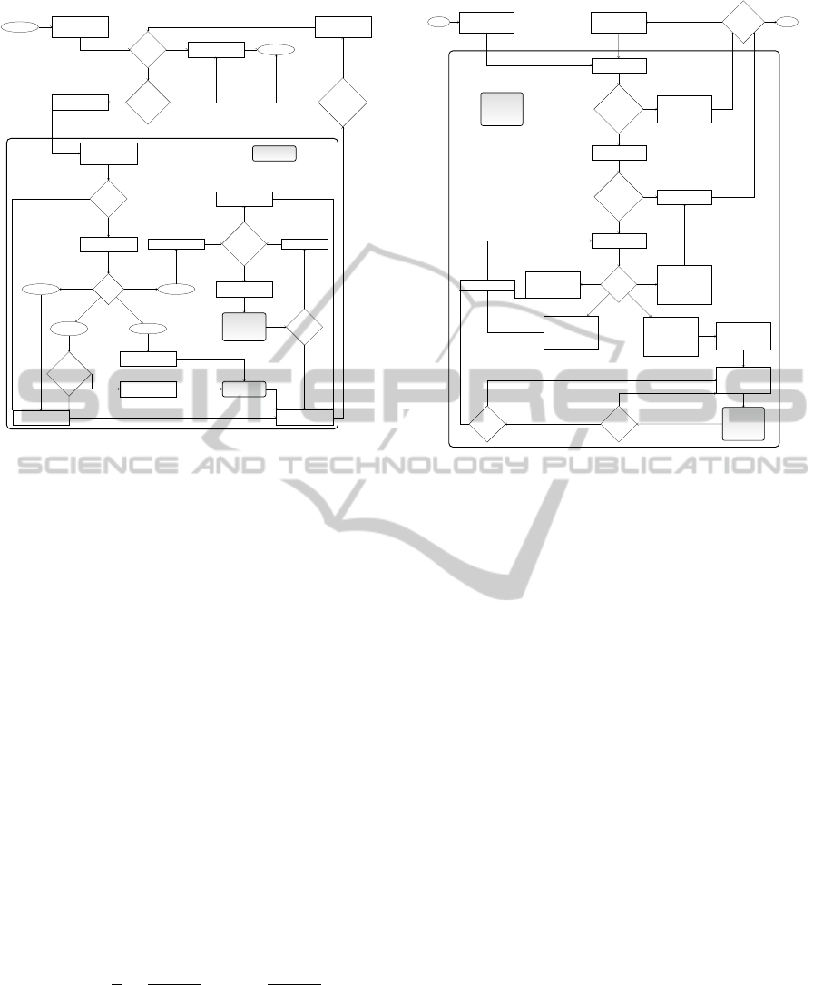
returns the partially formed substructure. Figure 3
gives a schematic overview on this inherently con-
trolled sampling strategy.
As regards this particular sampling strategy, the out-
side values can easily be omitted from the correspond-
ing formulae for defining the needed sampling prob-
abilities, since in any case they contribute the same
multiplicative factor to the distinct sampling proba-
bilities for mutually exclusive and exhaustive cases,
such that they finally do not influence the sampling
decision at all.
The correctness of this simplification can easily be
verified by considering a particular set ac
X
(i, j) of all
choices for (valid) derivations of intermediate symbol
BIOINFORMATICS 2012 - International Conference on Bioinformatics Models, Methods and Algorithms
70
Start folding of
R
i+1,j−1
:= R
h+1,l−1
(by adding pair i.j)
i.j could
close loop?
Sample loop type
closed by i.j
Type
Hairpin
Stacking
Take consecutive pair
h.l := (i + 1).(j − 1)
Bulge or
interior
Helix
possible on
R
i+1,j−1
?
Sample accessible pair
h.l (first h, then l)
Multiloop
Set k := 1 and l := i
kth helix
possible on
R
l+1,j−1
?
R
l+1,j−1
remains
single-stranded
Sample kth accessible
pair h.l (first h, then l)
Recursively
fold the kth
multiloop
substructure S
h,l
Further
helix?
Set k := k + 1
S
i+1,j−1
becomes
single-strand
Recursively fold
substructure S
h,l
Finish folding of R
i,j
(S
i,j
is now complete)
Helix
possible on
R
i,j
?
Sample free pair h.l
(first h, then l)
Further
helix?
Consider entire
input sequence
R
i,j
:= R
1,n
Start
S
i,j
becomes
single-strand
End
Overall
structure
S
1,n
folded?
Consider remaining
sequence fragment
R
i,j
:= R
j+1,n
no
yes
yes
no
no
yes
no
yes
no
yes
no
yes
no
yes
Recursively fold
substructure S
h,l
Figure 3: Flowchart for recursive sampling of an RNA sec-
ondary structure S
1,n
for a given input sequence r of length
n according to an inherently controlled strategy with pre-
determined order, similar to that of (Ding and Lawrence,
2003; Nebel and Scheid, 2011)).
X ∈ I
G
s
on sequence fragment R
i, j
, 1 ≤ i < j ≤ n,
which actually correspond to possible substructures
on R
i, j
. Under the assumption that the alternatives for
intermediate symbol X are X → Y and X → VW , the
(valid) mutually exclusive and exhaustive cases are
defined by:
acX(i, j) := acX
Y
(i, j) ∪ acX
VW
(i, j), (10)
where
acX
Y
(i, j) := {{0, p} | p 6= 0 for
p = β
X
(i, j) · α
Y
(i, j) · Pr
0
tr
(X → Y )} (11)
and
acX
VW
(i, j) := {{k, p} | i ≤ k ≤ j and p 6= 0 for
p = β
X
(i, j) · α
V
(i,k)α
W
(k + 1, j) · Pr
0
tr
(X → VW )}.
(12)
We then sample from the probability distribution in-
duced by acX(i, j) (conditioned on fragment R
i, j
),
which implies
1 =
∑
p∈acX(i, j)
p
z
=
β
X
(i, j)
z
∑
p∈acX(i, j)
p
β
X
(i, j)
(13)
for z :=
∑
p∈acX(i, j)
p, since β
X
(i, j) 6= 0 due to the def-
inition of acX(i, j).
4.2 Alternative Strategy
Unfortunately, the common sampling strategy from
Start folding of
R
start,end
(Further)
hairpin
possible on
R
start,end
?
Finish folding of
R
start,end
(unfolded positions
become unpaired)
Sample hairpin loop
S
ii,jj
on R
start,end
S
ii,jj
extendable
on
R
start,end
?
Finish folding of
substructure S
ii,jj
Sample extension of
S
ii,jj
on R
start,end
Extension
type
Stacking:
S
ii,jj
is extended by
adding enclosing base
pair(s)
Bulge or interior:
S
ii,jj
is extended by
adding a preceding or
a following
single-strand (or both)
Substructure of
multiple loop:
S
ii,jj
is extended by
adding a preceding
single-strand of
arbitrary length
Substructure of
exterior lo op:
S
ii,jj
is extended by
adding a preceding
single-strand of
arbitrary length
Update ii and jj
Update end
(must be indeed the
last position of the
multiloop)
Update start
(not necessarily the
first position of the
multiloop)
Recursively fold
new (paired)
substructure
S
ii,jj
on
R
start,end
Structure
type
Multiloop
complete?
Still exist
unfolded
fragments?
End
Take one of the
unfolded fragments
R
start,end
Take sole unfolded
fragment
R
start,end
:= R
1,n
Start
no
yes
no
yes
substructure of exterior loop
substructure of multiple loop
no
yes
yes
no
Recursively fold
new (paired)
substructure
S
ii,jj
on
R
start,end
Figure 4: Flowchart for recursive sampling of an RNA sec-
ondary structure S
1,n
for a given input sequence r of length
n according to a less restrictive strategy with extensively
more freedom (that requires dynamic validation of possible
random choices during the sampling process).
Section 4.1 lacks the ability to take full advan-
tage of the exact inside values
b
α
X
(i, j) = α
X
(i, j), for
X ∈ I
G
s
and j −i+1 ≤ W
exact
, obtained by employing
a particular mixed preprocessing variant according to
0 ≤ W
exact
< n. Particularly, the strategy in general
inevitably has to sample the first base pairs from cor-
responding conditional probability distributions for
rather large fragments R
i, j
with j − i + 1 > W
exact
,
which are indeed induced by approximated sampling
probabilities rather than exact ones. Therefore, we
worked out an alternative to this well-established
sampling strategy that obeys to contrary principles,
resulting in a reverse sampling direction.
Basically, a complete secondary structure S
1,n
for
a given input sequence r of length n can alternatively
albeit unconventionally be sampled in the following
(deliberately less controlled) way: Start with the en-
tire RNA sequence R
start,end
= R
1,n
and randomly
construct adjacent substructures (paired substructures
preceeded by potentially empty single-stranded re-
gions) of the exterior loop on the considered sequence
fragment R
start,end
(where the construction does not
follow a particular order, e.g. does not sample from
left to right), as long as no further paired substructure
can be folded. Any (paired) substructure on fragment
R
start,end
, 1 ≤ start ≤ end ≤ n, is created by sampling
a random hairpin loop (with closing base pair i. j, for
start < i < j < end) – here we can take advantage of
A n2 RNA SECONDARY STRUCTURE PREDICTION ALGORITHM
71

Table 1: Comparsion of the considered sampling strategies (for an arbitrary input sequence of length n).
Aspect Conventional Strategy Alternative Strategy
Preprocessing time O(n
3
) for exact calculations,
O(n
2
) for approximate variant,
O(n
2
) with constant W
exact
≥ 0
O(n
3
) for exact calculations,
O(n
2
) for approximate variant,
O(n
3
) with constant W
exact
≥ 0
Constraints None Constant max
hairpin
, max
bulge
and max
strand
Characteristics and
course of action
Inherently controlled, ordered:
- substructures from left to right,
- sampling proceeds “inwards”:
construction of substructure S
i, j
starts
by considering R
i, j
and ends by gener-
ating an unpaired region (usually a hair-
pin loop)
Extensively more freedom, less restrictive:
- substructures in arbitrary order,
- sampling proceeds “outwards”:
construction of new substructure on unfolded frag-
ment R
start,end
starts with random hairpin loop
which is extended to a complete and valid (paired)
substructure S
i, j
on R
start,end
Benefits of sam-
pling direction
(Sub)structures are folded in accor-
dance with the generation of the cor-
responding (unique leftmost) derivation
(sub)tree by the underlying SCFG
Takes more advantage of inside probabilities for
shorter fragments containing less approximated
terms and thus less inaccuracies (although this po-
tential is narrowed by the outside values for which
the contrary holds)
Function of outside
values
Not considered (do not influence sam-
pling distributions)
1) “Normalize” sampling probabilities
2) Ensure valid extensions
Identification of
valid choices
Not required (all possible choices are
principally valid)
Dynamic checking required (due to dependence on
previously folded substructures)
Folding time O(n
2
) O(n
2
) with larger constants
Overall time com-
plexity for MP pre-
dictions
O(n
3
) with exact variant,
O(n
2
) with constant W
exact
≥ 0 or in
completely approximated case
O(n
3
) in case of exact computations or mixed vari-
ants according to W
exact
≥ 0,
O(n
2
) only in completely approximated case
exact inside values from a mixed preprocessing since
most likely i and j are close – and extending it (to-
wards the ends of R
start,end
) by successively drawing
closing base pairs. During this extension, basically all
known substructures (stacked pairs, bulges, interior
and multibranched loops, that obey to certain restric-
tions which will be discussed later) may be folded,
where each substructure (e.g. multiloop) has to be
completed before its closing base pair is added and the
corresponding helix can actually be further extended.
The process of folding a particular paired substructure
ends with a complete and valid paired structure (of the
currently folding multiloop or of the exterior loop), ei-
ther with or without a directly preceeding unpaired re-
gion, both on the considered fragment R
start,end
. Fig-
ure 4 gives a schematic overview on this inside-out
fashion sampling strategy.
Note that in order to ensure that all sampled sub-
structures can be successfully folded, especially in
the case of multiloops, we have to take care that at
any point, the strategy may only draw such random
choices that do not make it impossible to success-
fully finish the currently running construction process
(of a particular loop). As this strongly depends on
the actual positions and types of all previously folded
paired substructures, the algorithm obviously needs to
dynamically determine the respective set of all valid
choices (during the sampling process itself) before
a corresponding probability distribution (needed for
drawing a particular random choice) can be derived.
This, however, may cause severe problems as re-
gards the time complexity for randomly sampling the
next extension (or base pair). Nevertheless, in or-
der to guarantee that the worst-case time complex-
ity for drawing any random choice remains in O(n),
we only need to impose a few restrictions concerning
the lengths of single-stranded regions in some types
of loops. In detail, we have to consider a maximum
allowed number of nucleotides in unpaired regions
of hairpin loops (max
hairpin
), bulge or interior loops
(max
bulge
), and multiloops (max
strand
)
5
For example, if X ∈ I
G
s
generates hairpin loops,
then the set of all possible hairpin loops that can be
validly folded on sequence fragment R
start,end
is given
by
pcHL(start, end) :=
{i, j, p} |
start + min
hel
≤ i ≤ j ≤ end − min
hel
and
i + min
HL
− 1 ≤ j ≤ i + max
hairpin
− 1 and
R
i−min
hel
, j+min
hel
not folded and
p =
b
β
X
(i, j) ·
b
α
X
(i, j) 6= 0
. (14)
Obviously, max
hairpin
indeed ensures that
5
Note that these restrictions are not as severe as it may
seem, since for example choosing the constant value 30 (as
also done by many MFE based prediction algorithms) for all
three parameters can be expected to hardly have a negative
impact on the resulting sampling quality.
BIOINFORMATICS 2012 - International Conference on Bioinformatics Models, Methods and Algorithms
72

pcHL(start, end) can be computed in O(n) time.
Finally, it should be noted that this sampling strategy
needs to additionally consider outside probabilities,
for two reasons: First, for “normalizing” the result-
ing sampling probabilities. This is due to the fact that
the different possible choices {i, j, p} usually imply
substructures S
i, j
of different lengths j − i + 1, such
that only p =
b
α
X
(i, j) ·
b
β
X
(i, j) ensures that the prob-
abilities of all possible choices are of the same order
of magnitude and hence imply a reasonable probabil-
ity distribution for drawing a random choice. Sec-
ond, the outside values are required for guaranteeing
that sampled substructures can be validly extended.
This means that only such hairpin loops and exten-
sions (implying a surrounding base pair i. j) may be
sampled that can actually lead to the generation of a
corresponding valid helix.
We conclude this section by referring to Table 1
that summarizes the main differences of both sam-
pling variants.
5 APPLICATIONS
First, the sampling results shown in Figure 5 indicate
that for the common sampling strategy, considering
a window of constant size W
exact
(chosen to cover
the size of hairpin-loops) with a mixed preprocess-
ing variant, actually yields a slight improvement of
the resulting sampling quality, where the same time
requirements are needed for generating the respective
sample sets.
Contrary to this observation, Figure 6 demon-
strates that when employing our alternative sampling
strategy, the corresponding results are not signifi-
cantly different for the completely approximate pre-
processing variant and for a mixed version on the ba-
sis of a constant value for W
exact
. Thus, to our surprise
it does not matter if we consider a constant window
for exact calculations or simply approximate all in-
side and outside values, which is not only an interest-
ing observation itself, but also fortunately prevents us
from having to deal with an undesirable trade-off be-
tween reducing the worst-case time complexity (by a
linear factor) and sacrificing less of the resulting sam-
pling quality. In fact, this means we may (without re-
sulting significant quality losses) always use the more
efficient approximative preprocessing variant in order
to reduce the worst-case time complexity of the over-
all sampling algorithm.
However, all profiles perfectly demonstrate that
due to the noisy ensemble distribution caused by ap-
proximating the highly relevant sequence-dependent
0
10
20
30
40
50
60
70
0.0
0.2
0.4
0.6
0.8
1.0
Nucleotide Position
Probability
Hplot
Figure 5: Sampling results for E.coli tRNA
Ala
, derived with
the common strategy (under the assumption of min
hel
=
2 and min
HL
= 3), where we used sample size 100,000,
10,000 and 1,000 for W
exact
= −1 (no window, thick gray
lines), W
exact
= 30 (moderate window, thick dotted darker
gray lines) and W
exact
= +∞ (complete window, thin black
lines), respectively.
0
10
20
30
40
50
60
70
0.0
0.2
0.4
0.6
0.8
1.0
Nucleotide Position
Probability
Hplot
Figure 6: Sampling results corresponding to those of Fig-
ure 5, obtained by employing the alternative sampling strat-
egy.
emission probabilities, the resulting sample sets usu-
ally contain many foldings that are rather unlikely ac-
cording to the exact distribution for the considered in-
put sequence. For this reason, it can not be recom-
mended to employ one of the following otherwise rea-
sonable construction schemes for deriving predictions
according to the entire sample set: we should rather
neither predict γ-MEA nor γ-centroid structures of the
generated sample set as defined in (Nebel and Scheid,
2011), since those effectively reflect the overall be-
havior of the sample set. Those predictions must any-
way be considered inappropriate choices in our case,
since their computation requires O(n
3
) time, which
would inevitably undo the time reduction reached by
approximating. Nevertheless, we can without signif-
icant losses in performance (without increasing the
worst-case time complexity of the overall algorithm)
identify the MP structure of the generated sample
6
, in
strong analogy to traditional SCFG approaches. Since
for this selection principle, we can actually rely on the
exact distribution of feasible structures
7
, this seems to
6
The probability of each structure can either be deter-
mined on the fly while sampling, multiplying the probabili-
ties of the production rules which correspond to the respec-
tive sampling decisions, and otherwise – since the under-
lying SCFG from (Nebel and Scheid, 2011) is unambigu-
ous – are computable in O(n
2
) time making use, e.g., of an
Earley-style parser.
7
Note that the probability for a particular folding of a
given RNA sequence is equal to a product of (different pow-
A n2 RNA SECONDARY STRUCTURE PREDICTION ALGORITHM
73

be the right choice indeed.
On the basis of a series of experiments, we observed
that stability in resulting predictions and a competi-
tive prediction accuracy can only be reached by in-
creasing the sample size, especially in the case of
complete approximation for the preprocessing step
and sampling according to the alternative strategy in-
troduced in Section 4.2. That is, more candidate struc-
tures ought to be generated for guaranteeing that the
resulting MP predictions are reproducible (by inde-
pendent runs for the same input sequence) and of
hight quality. This negative effect is considerably
lowered by using (larger) constant values of W
exact
≥
0, and is actually less recognizable when employing
the conventional sampling strategy recapped in Sec-
tion 4.1.
0
20000
40000
60000
80000
100000
0.5
0.6
0.7
0.8
0.9
1.0
Sample Size
Sensitivity
0
20000
40000
60000
80000
100000
0.5
0.6
0.7
0.8
0.9
1.0
Sample Size
Specificity
0
20000
40000
60000
80000
100000
0.5
0.6
0.7
0.8
0.9
1.0
Sample Size
Sensitivity
0
20000
40000
60000
80000
100000
0.5
0.6
0.7
0.8
0.9
1.0
Sample Size
Specificity
Figure 7: Sensitivity and specificity of predictions as a func-
tion of sample size derived for E.coli tRNA
Ala
. Top (bot-
tom) lines show the common (alternative) sampling strat-
egy.
Figure 7 shows the averaged sensitivities and
specificities obtained for 50 independent runs of con-
tinuously sampling secondary structures taking the so
far most probable one as the actual prediction (which
determines sensitivity and specificity for the actual
sample size). We observe that when making use of
approximate probabilities sample sizes about 40 to
50 times as large as for a precise preprocessing are
needed to generate competitive predictions. Thus, for
ers of the diverse) transition and emission probabilities (ac-
cording to the corresponding derivation tree), which means
it depends only on the exact trained parameter values of the
underlying SCFG.
a naive implementation the speedup gained by ap-
proximation may partly be lost. However, unlike pre-
diction algorithms using dynamic programming, sam-
pling can easily be parallelized. Making use of a grid
environment where today one may assume a proces-
sor to have about 8 cores, a grid of size 5 or 6 com-
puters is sufficient to compensate the increased sam-
ple size. Furthermore, since we only make use of
the most probable sampled structure for our predic-
tion, sampling can be done in-place, storing in each
core only the best structure seen so far. This re-
duces the memory requirements and keeps the com-
munication costs rather moderate since it is finally
only necessary to gather m structures from m cores
and select the best. We performed a series of exper-
iments, making use of Mathematica’s parallel com-
putation features, which proved that the overall pro-
cess scales linearly in the number of cores used with
a non-measurable communication overhead. This fi-
nally proves the applicability of our approach provid-
ing a factor n speedup compared to established predic-
tion tools but still maintaining the limits implied by a
quadratic memory consumption (in our case used to
store parameter values).
6 CONCLUSIONS
The major advantage of the presented approximative
method is that it is more efficient than all other mod-
ern prediction algorithms (implemented in popular
tools like Mfold (Zuker, 2003), Vienna RNA (Ho-
facker, 2003), Pfold (Knudsen and Hein, 2003),
Sfold (Ding et al., 2004) or CONTRAfold (Do et al.,
2006)), reducing the worst-case time complexity by
a linear factor, such that the time and space require-
ments are both bounded by O(n
2
). However, a poten-
tial drawback lies in the observation that the overall
quality of generated samples decreases (as indicated
by probability profiling for specific loop types), which
is due to the approximated ensemble distribution. As
a consequence, we usually need to use larger sample
sizes for obtaining a competitive prediction accuracy
and stable predictions, i.e., more candidate structures
for a given input sequence have to be generated to
ensure that the approximation method outputs rather
identical predictions in independent runs for that se-
quence. According to our experiments, an efficient
implementation that really takes advantage of the ac-
celerated preprocessing (3.7 compared to 49 seconds
for our proof-of-concept implementation in Wolfram
Mathematica) but handles large sample sizes can be
obtained by parallelization.
Note that all results presented in this article have been
BIOINFORMATICS 2012 - International Conference on Bioinformatics Models, Methods and Algorithms
74

derived with a purposive proof-of-concept implemen-
tation of the described methods. A more sophisti-
cated tool will be realized in the future, hoping that
the proposed prediction approach proves capable of
yielding acceptable accuracies even for such types of
RNAs whose molecules imply a great variety of struc-
tural features (due to large sequence lengths). In fact,
we here only considered exemplary applications for
one particular tRNA molecule in order to get positive
feedback that (at least) the MP predictions obtained
via approximated SCFG based sampling can be of
high quality. Accordingly, more general experiments
are needed, e.g., in connection with RNA molecules
of sizes n = 3000 − 30000 (for which the memory
constraints of our approach are not restrictive assum-
ing 1GB of memory for each core) and where long
distance base pairs in a global folding are of interest.
In such a scenario the proposed algorithm could be
the method of choice provided it performs similarly
well.
This line of research is work in progress, but we
found the first impressions presented within this note
so motivating that we wanted to share them with the
scientific community already at this point, primarily
because this work leaves a number of open questions
that may be inspiration for further research of other
groups. For instance, recall that we used a sophis-
ticated SCFG (representing a formal language coun-
terpart to the thermodynamic model applied in the
Sfold program) as probabilistic basis for the consid-
ered sampling strategies. However, it would also be
possible to employ other SCFG designs, for example
one of the commonly known lightweight grammars
from (Dowell and Eddy, 2004). This might of course
yield at least noticeable if not significant changes in
the resulting sampling quality, which could be an in-
teresting subject to be explored.
It should also be noted that a similar approxima-
tive approach could potentially be considered when
attempting to reduce the worst-case time complexity
of the sampling extension of the PF approach. In fact,
since sequence information is incorporated into the
used (equilibrium) PFs and corresponding sampling
probabilities only in the form of particular sequence-
dependent free energy contributions, it seems reason-
able to believe that the time complexity for the for-
ward step (preprocessing) could possibly be reduced
by a linear factor to O(n
2
) when using some sort
of approximated (averaged) free energy contributions
that do not depend on the actual sequence (but con-
tain as much sequence information as possible), in
analogy to the approximated preprocessing step (in-
side and outside calculations) considered in this work,
where we eventually only had to use averaged emis-
sion terms instead of the exact emission probabilities
in order to save time.
REFERENCES
Akutsu, T. (1999). Approximation and exact algorithms for
RNA secondary structure prediction and recognition
of stochastic context-free languages. J. Comb. Optim.,
3(2–3):321–336.
Backofen, R., Tsur, D., Zakov, S., and Ziv-Ukelson, M.
(2011). Sparse RNA folding: Time and space efficient
algorithms. Journal of Discrete Algorithms, 9:12–31.
Ding, Y., Chan, C. Y., and Lawrence, C. E. (2004). Sfold
web server for statistical folding and rational design
of nucleic acids. Nucleic Acids Research, 32:W135–
W141.
Ding, Y. and Lawrence, C. E. (2003). A statistical sam-
pling algorithm for RNA secondary structure predic-
tion. Nucleic Acids Research, 31(24):7280–7301.
Do, C. B., Woods, D. A., and Batzoglou, S. (2006).
CONTRAfold: RNA secondary structure predic-
tion without physics-based models. Bioinformatics,
22(14):e90–e98.
Dowell, R. D. and Eddy, S. R. (2004). Evaluation of sev-
eral lightweight stochastic context-free grammars for
RNA secondary structure prediction. BMC Bioinfor-
matics, 5:71.
Frid, Y. and Gusfield, D. (2010). A simple, practical and
complete O(n
3
/log(n))-time algorithm for RNA fold-
ing using the Four-Russians speedup. Algorithms for
Molecular Biology, 5(1):5–13.
Hofacker, I., Fontana, W., Stadler, P., Bonhoeffer, S.,
Tacker, M., and Schuster, P. (1994). Fast folding and
comparison of rna secondary structures (the Vienna
RNA package). Monatsh Chem., 125(2):167–188.
Hofacker, I. L. (2003). The vienna RNA secondary structure
server. Nucleic Acids Research, 31(13):3429–3431.
Knudsen, B. and Hein, J. (1999). RNA secondary structure
prediction using stochastic context-free grammars and
evolutionary history. Bioinformatics, 15(6):446–454.
Knudsen, B. and Hein, J. (2003). Pfold: RNA sec-
ondary structure prediction using stochastic context-
free grammars. Nucleic Acids Research, 31(13):3423–
3428.
McCaskill, J. S. (1990). The equilibrium partition function
and base pair binding probabilities for RNA secondary
structure. Biopolymers, 29:1105–1119.
Nebel, M. E. and Scheid, A. (2011). Evaluation of a so-
phisticated SCFG design for RNA secondary structure
prediction. Submitted.
Wexler, Y., Zilberstein, C., and Ziv-Ukelson, M. (2007). A
study of accessible motifs and RNA folding complex-
ity. Journal of Computational Biology, 14(6):856–
872.
Zuker, M. (1989). On finding all suboptimal foldings of an
RNA molecule. Science, 244:48–52.
Zuker, M. (2003). Mfold web server for nucleic acid fold-
ing and hybridization prediction. Nucleic Acids Res.,
31(13):3406–3415.
A n2 RNA SECONDARY STRUCTURE PREDICTION ALGORITHM
75
