NONLINEAR MAPPING BY CONSTRAINED CO-CLUSTERING

Rodolphe Priam

, Mohamed Nadif

and G´erard Govaert

S3RI, University of Southampton, University Road, SO17 1BJ, Southampton, U.K.

LIPADE, Universit´e Paris Descartes, 45 rue des Saints P`eres, 75006 Paris, France

HEUDIASYC, Universit´e de Technologie de Compi`egne, 60205 Compi`egne, France

Keywords:

Generative topographic mapping, Latent block model, Contingency table, Clustering.

Abstract:

The latent block model is an efﬁcient alternative to the mixture model for modelling a dataset when the number

of rows or columns of the data matrix studied is large. For analyzing and reducing the spaces of a matrix, the

methods proposed in the litterature are most of the time with their foundation in a non-parametric or a mixture

model approach. We present an embedding of the projection of co-occurrence tables in the Poisson latent

block mixture model. Our approach leads to an efﬁcient way to cluster and reduce this kind of data matrices.

1 INTRODUCTION

Contingency tables, or co-occurrence matrices, are

found in diverse domains. In these matrices each cell

is a cross-product of two categorical variables I (n cat-

egories) and J (d categories.) The cells contain the

number of occurrences for the corresponding cross-

categories. Contingency tables appear in information

retrieval (Deerwester et al., 1990) and document clus-

tering (Hofmann, 1999), where I may correspond to

a corpus of documents, J to a set of words, and so

the frequency denotes the number of occurrences of

a word in a document. Other examples from data

mining, preference analysis, etc., show that analyzing

contingency tables is in fact a very common and fun-

damental aspect of data analysis. Contingency tables

are usually analyzed using one of the many categori-

cal data analysis methods available in the literature.

When the data matrix is large, a clustering can

give a quicker and easier access to the data con-

tent than a method for reducing the dimensionality

of the features. Combining clustering and reduction

for mapping clusters rather than rows or columns is

therefore an interesting requirement for data analysis.

One way to fulﬁll this purpose is by showing the clus-

ters on a map after clustering the data by an ad’hoc

algorithm and reducing the feature space, both sep-

arately. Alternatively, the Kohonen’s self-organizing

map (SOM) (Kohonen, 1997) is such that the clus-

tering and the mapping of the clusters take place si-

multaneously while providing one ﬁnal unique map.

The SOM algorithm is not derived exactly through the

optimization of an objective function, and several pa-

rameters have to to be set empirically.

A probabilistic model for SOM is appealing for

several reasons, the principal one is that a parametric

model is ﬂexible and scalable when deﬁned properly.

We are interested in proposing an efﬁcient paramet-

ric model for a bidimensional mapping of the clusters

of I for a contingency table. Generative Topographic

Mapping (GTM) (Bishop et al., 1998) is a parametric

SOM with a number of advantages compared to the

standard SOM. It re-formulates SOM by embedding

the constraints of vicinity for the clusters in a Gaus-

sian mixture model (GMM) (McLachlan and Peel,

2000). Classical mixture models, and in particular

GMM, are generally not efﬁcient for large datasets,

and this is also true of GTM. One possible alternative

to a clustering of rows or columns is a co-clustering

approach that clusters the two dimensions of a ma-

trix simultaneously and efﬁciently, with a competitive

small number of parameters.

Here we turn to the latent block model (see (Go-

vaert and Nadif, 2003)) with constraints in order to

simultaneously cluster and visualize the clusters. In

contrast to previous works like for instance (Kab´an

and Girolami, 2001), (Hofmann, 2000) or (K´aban,

2005), the proposed method is parsimonious since the

number of parameters remains constant when the size

of the data matrix increases.

The paper is organized as follows. In Section 2 we

review co-clustering for co-occurrence tables, and de-

scribe a Poisson latent block model (PLBM) (Govaert

and Nadif, 2010). We add constraints in the model

Priam R., Nadif M. and Govaert G. (2012).

NONLINEAR MAPPING BY CONSTRAINED CO-CLUSTERING.

In Proceedings of the 1st International Conference on Pattern Recognition Applications and Methods, pages 63-68

DOI: 10.5220/0003764800630068

 SciTePress

and propose an algorithm for the estimation of the pa-

rameters. In section 3 we present an evaluation of our

new method named BlockGTM. Finally, the conclu-

sion summarizes the advantages of our contribution.

2 BLOCK EM MAPPING

In latent block model (LBM) the n × d random vari-

ables generating the observed x

cells of the data ma-

trix are assumed to be independent, once z and w are

ﬁxed where the set of all possible assignments w of J

(resp. z of I) is denoted W (resp. Z ). The data matrix

x is therefore a set of cells:

,...,x

rather than the sample of d-dimensional vectors in the

more classical mixture setting. The two sets of pos-

sible assignments w and z cluster the cells of the ma-

trix x into a number of contiguous, non-overlapping

blocks. A block kℓ is deﬁned as the set of cells

= k,w

= ℓ}. The binary classiﬁcation matrix

z = (z

)

n×g

is such that

∑

k=1

= 1 and z

= 1 in-

dicates the component of the row i, and similarly for

the columns with w = (w

jℓ

)

d×m

The following decomposition is obtained (Gov-

aert and Nadif, 2003) by independence of z and w,

by summing over all the assignments:

LBM

(x;θ) =

∑

(z,w)∈Z ×W

∏

i,k

∏

j,ℓ

jℓ

ℓ

∏

i, j,k,ℓ

ϕ(x

;α

kℓ

)

jℓ

where ϕ(.;α

kℓ

) is a density function deﬁned on the set

of reals R and {α

kℓ

} are unknown parameters. The

vectors of the probabilities p

and q

ℓ

that a row and a

column belong to the k-th component and to the ℓ-th

component are respectively denoted p = (p

,..., p

)

and q = (q

,...,q

). The set of parameters is denoted

θ and is compound of p and q plus α which aggre-

gates all the α

kℓ

. Hereafter, to simplify the notation,

the sums and the products relating to rows, columns

or clusters will be subscripted respectively by the let-

ters i, j or k, ℓ without indicating the limits of varia-

tion, which are implicit. Next, PLBM is described for

contincency tables and the constraints are added.

2.1 Poisson Latent Block Model

For co-occurrence tables, PLBM assumes that the

observed values x

in a block kℓ are drawn from

a Poisson distribution P(λ

kℓ

) with parameter λ

kℓ

where the effects µ = (µ

,...,µ

) and ν =

(ν

,...,ν

) are assumed equal to the margin totals

{µ

∑

;1 ≤ i ≤ n} and {ν

∑

;1 ≤ j ≤ d}.

Then ϕ for the block kℓ is deﬁned as follows:

ϕ(x

;µ

,ν

,α

kℓ

) =

exp(−µ

kℓ

)(µ

kℓ

)

Given that x

∈ N

, the unknown parameter α

kℓ

the block kℓ is in [0;1], since x

< µ

. The set of

parameters θ of the model can be estimated by maxi-

mizing the log-likelihood:

L(x;θ) = log f

LBM

(x;θ).

2.2 Constrained Parameters

To induce a quantization with a large number of clus-

ters, the probabilities p

and q

ℓ

are ﬁxed and equipro-

portional such that {p

= 1/g;1 ≤ k ≤ g} and {q

ℓ

1/m;1 ≤ ℓ ≤ m}. The parameters of the Poisson LBM

are parameterized with the ﬁxed vectors {ξ

} deﬁned

hereafter for the mapping of I, and the unknown vec-

tors {w

ℓ

∈ R

,1 ≤ ℓ ≤ m, h ∈ N

∗

} because α

kℓ

is de-

pendent on the index k and ℓ. The parameters {w

ℓ

}

are estimated by maximum likelihood. For deﬁning

the vectors {ξ

}, it is considered the bidimensional

coordinates:

S = {s

= (s

);k = 1, ...,g},

from the nodes of a regular mesh discretizing the

square where the data are projected [−1;1] × [−1;1].

S is similar to the set of nodes of SOM. As in GTM,

each coordinate s

is nonlinearly transformed by h ba-

sis functions φ such as:

= Φ(s

) = (φ

),φ

),. ..,φ

))

where each basis function φ is a kernel-like function:

φ(s

) ∝ exp[−||s

− µ

/2ν

with a mean center µ

∈ R

and a standard deviation

. It is then considered the inner products:

ℓ

;1 ≤ k ≤ g,1 ≤ ℓ ≤ m}.

To map the inner product (w

ℓ

∈ R) onto its cor-

responding parameter (α

kℓ

∈ [0;1]) it is used a sig-

moidal function σ(.) as in (Girolami, 2001) such that

for 1 ≤ k ≤ g, 1 ≤ ℓ ≤ m, we have:

kℓ

= σ(w

ℓ

) =

exp(w

ℓ

)

1+ exp(w

ℓ

)

The relative ordering of the coordinates {s

);k = 1, ..., g} remains, at least locally, after

the transformation. The reduced g × m matrix α in

PLBM is replaced by an h× m matrix:

Ω = [w

|···|w

ICPRAM 2012 - International Conference on Pattern Recognition Applications and Methods

The model remains parsimonious because h is small,

less than half of one hundred in practice.

Below we present an algorithm for the estima-

tion of the parameters θ = Ω, the matrix for the con-

straints. The optimization problem is slightly differ-

ent from the unconstrained case, as we shall explain

in the next section.

2.3 Parameter Estimates

For the proposed model with the introduced con-

straints, we aim to address the problem of parameters

estimation by a maximum likelihood (ML) approach

such that:

θ = argmax

L(x;θ).

For ﬁnding a suitable value of θ for the constrained

PLBM, the Block EM (BEM) (Govaert and Nadif,

2005) results in the following criterion (denoted

Q for

short) which is maximized iteratively:

BlockGTM

(θ,θ

(t)

)

∑

i, j,k,ℓ

(t)

jℓ

logϕ(x

;α

kℓ

)

∑

i, j,k,ℓ

(t)

jℓ



logα

kℓ

− µ

kℓ



+ cte

∑

k,ℓ

(t)

kℓ

logα

kℓ

− µ

(t)

ℓ

kℓ

) + cte. (1)

Here cte is a constant independent of the parameters,

the index (t) permits to denote a current estimation

of a parameter or a function of the parameters. It is

also denoted y

(t)

kℓ

∑

i, j

(t)

jℓ

, µ

(t)

∑

(t)

, and

(t)

ℓ

∑

(t)

jℓ

, while given θ

(t)

, the quantities c

(t)

(resp. d

(t)

jℓ

) are the posterior probabilities that a row

(resp. a column) belongs to the block kℓ. Here, the

posterior probabilities are estimated by using the de-

pendent equations:

(t)

∝ exp

∑

jℓ

(t)

jℓ

logϕ(x

;α

(t)

kℓ

)

, (2)

(t)

jℓ

∝ exp

∑

(t)

logϕ(x

;α

(t)

kℓ

)

. (3)

At the ML, they are denoted { ˆc

} and {

jℓ

}. The pa-

rameters are estimated in an iterative way. The BEM

algorithm proceeds by an alternated maximization of

Q. At each iteration the posterior probabilities {c

}

and {d

jℓ

} are evaluated for all rows and all columns,

and just after the maximization of the function

Q is

obtained with respect to the parameters. As a re-

mark, this induces a maximization with a variational

approximation at each iteration. Another approxima-

tion of the resulting criterion

Q is also required at the

maximization step as explained in the following para-

graphs.

2.4 Algorithm

The algorithm for maximizing

Q proceeds iteratively

by increasing an approximation of the log-likelihood

at each step. At the Maximization step we estimate

the next current value for θ

(t+1)

by:

(t+1)

= argmax

Q(θ|θ

(t)

Let us have ε a small positive real. The algorithm for

ﬁnding the maximum likelihood solution is given in

Figure 1 (see Appendix for

(t)

ℓ

and

(t)

ℓ

Learning algorithm for BlockGTM:

- Initialization:

Initialize {c

(0)

}, {d

(0)

jℓ

} and Ω

(0)

- E-Step:

Compute {c

(t)

} by (2), and {d

(t)

jℓ

} by (3) in a

loop.

- M-Step:

Compute the new parameters for ℓ = 1, . . . , m

(t+1)

ℓ

= w

(t)

ℓ

(t)

ℓ

−1

∇

(t)

ℓ

, (4)

with ∇

(t)

ℓ

by (5) and

(t)

ℓ

by (6).

- End:

If |Ω

(t+1)

− Ω

(t)

| < ε then stop else return E-

Step.

Figure 1: Iterations for BlockGTM.

Next, we evaluate the performance of BlockGTM for

several real datasets.

3 NUMERICAL EXPERIMENTS

In order to test the proposed method, we construct the

bidimensional projections of the obtained clusters by

the proposed method for four textual datasets.

3.1 Bi-dimensional Mapping

The set of bidimensional coordinates S for the g clus-

ters are used to ﬁnd the ﬁnal projection ˆs

of each

category i in the latent space. When a row i has a

higher posterior probability ˆc

for a cluster k then it

belongs to this cluster and the label for the i-th row

NONLINEAR MAPPING BY CONSTRAINED CO-CLUSTERING

is estimated by ˆz

= k. This same row can then be

represented at the bidimensional coordinates ˆs

MAP

ˆz

= (s

ˆz

)

. By performing this procedure for

each row i, the model builds a reduced view of the

n categories of I. Moreover, when two nodes have

their coordinates s

and s

′

near in the latent space,

their corresponding clusters should have similar pa-

rameters α

kℓ

and α

′

ℓ

, so their corresponding contents

should be also similar. A fuzzy projection can be ob-

tained by computing an average position of each row

i from its posterior probabilities ˆc

. This is written

ˆs

∑

k=1

ˆc

)

. If the vector of probabilities

( ˆc

, ˆc

,··· , ˆc

) is binary, then the row i is in the clus-

ter ˆz

, and ˆs

= ˆs

MAP

. This is generally the case for

GTM for a large part of the dataset. In the experimen-

tal part, it is constructed only a tabular view after bi-

narizing these vectors of probabilities, except a small

illustrative example.

3.2 Datasets

The characteristics of the four real datasets are de-

scribed below.

- N4. This dataset is composed of 400 documents

selected from a textual corpus of 20000 usenet

posts from 20 original newsgroups. From each

group among the 4 retained, 100 posts are selected

and 100 terms are ﬁltered by mutual information

(Kab´an and Girolami, 2001).

- Binary

. This dataset in (Slonim et al., 2000)

consists of 500 posts separated into two clus-

ters for the newsgroups talk.politics.mideast and

talk.politics.misc. A preprocessing was carried

out by the authors to reduce the number of words

by ignoring all ﬁle headers, stop words and nu-

meric characters. Moreover, using the mutual in-

formation, the top 2000 words were selected.

- Multi5

. This dataset in (Slonim et al., 2000),

consists of 500 posts separated into ﬁve clus-

ters comp.graphics, sci.space, rec.motorcycles,

res.sports.baseball and talk.politics.mideast. The

same pre-processing than for Binary

was per-

formed.

- C3. This dataset in (Dhillon et al., 2003), also

known as Classic3, is often used as a benchmark

for co-clustering. This dataset is a contingency

table of size 3891 x 4303 and it is compound of

three classes denoted Medline, Cisi and Cranﬁeld

as in the larger complete data sample not consid-

ered here.

These four datasets studied in our experiments are

of increasing size.

3.3 Results

Table 1 summarizes the characteristics of the datasets

and the parameters for BlockGTM. The four con-

structed maps are squares of size g = 9 × 9 for the

clustering in rows, while the number of clusters m in

columns and the dimension h were chosen after a few

tries. Each map is represented as following. For each

k-th cluster, a barplot corresponding to the true labels

of the data in the cluster is constructed at position s

after ﬁtting the model. The results are shown in Fig-

ure 2 for Multi5

and C3. So, for a given dataset

the map shows a matrix of 9 × 9 barplots such as if

two nodes are close on the latent space they should

have similar barplots. This is a tabular view of the

data (categories I) which conﬁrms also that the near-

est clusters have their texts with similar topics as ex-

pected.

Table 1: Summary where n×d is the size of the contingency

table, m is the number of clusters in columns, h is the num-

ber of basis functions, and E

(resp. E

) is the accuracy in

percent from BlockGTM (resp. PLBM).

Data n d m h E

N4 400 100 10 12 96.5 93.4

Binary

400 100 10 19 91.2 92.4

Multi5

500 2000 20 19 90.6 89.0

C3 3891 4303 20 28 99.1 99.3

In this section we are interested on measuring how

well the co-clustering can reveal the inherent struc-

ture of a given textual dataset. We consider the ac-

curacy which is usually derived from the confusion

matrix or the cluster purity. Speciﬁcally, we mea-

sure the quality of the clustering for the obtained clus-

ters comparatively to the real categories of the docu-

ments. The columns E

and E

of Table 1 give, in

percent, the accuracy obtained respectively for Block-

GTM and PLBM initialized with the ﬁnal parameters

of BlockGTM.

- For N4, the categories of I are projected by the

Correspondence Analysis (CA) method (Benze-

cri, 1980). The coordinates from CA are used

to compute the positions of the mean centers in

a 3-dimensional space thanks to the quantities ˆc

Figure 3 shows the result. It is interesting to note

that the original mesh compound of the nodes S

in the latent space is easily recognized in this 3-

dimensional space. Here each class is quantized

by a subset of clusters from the map, and the sub-

set usually includes only data with their corre-

sponding projections close in the space of projec-

tion as expected.

- For C3, the proposed method extracts the origi-

ICPRAM 2012 - International Conference on Pattern Recognition Applications and Methods

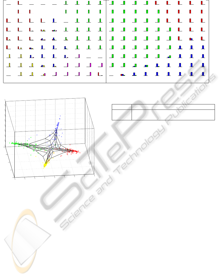
(a) (b)

Figure 2: The result from the proposed method for the datasets (a) Multi5

, and (b) C3.

−2

−1

−2

−1.5

−1

−0.5

0.5

1.5

−1

−0.5

0.5

1.5

2.5

3.5

Figure 3: A result from BlockGTM for N4 in the 3-

dimensional space of the projection with the 3 ﬁrst principle

factorial directions of CA.

nal clusters almost correctly. The accuracy of the

method is 1 − 33/3891 = 99.15%, while the co-

clustering based on (Dhillon et al., 2003) has an

accuracy of 97.74 = 1− 88/3891 so the obtained

error is smaller. The macro-clustering comes after

a ﬁner clustering and is better able to separate the

different classes.

- For Binary

and Multi5

, Table 2 reports the

resulting accuracies for BlockGTM, PLBM,

double

(Slonim et al., 2000), and IDC-15 (El-

yaniv and Souroujon, 2001). This helps for the

comparison between the different results. Despite

a slightly different error rate, the proposed method

is able to map the whole datasets and separate the

natural classes. The main difference with the al-

ternative approaches is not only the efﬁcient co-

clustering, but also the capacity to provide a quick

Table 2: Accuracy for BlockGTM, PLBM, IB

double

, IDC.

BlockGTM PLBM IB

double

IDC-15

Binary

91.2 92.4 70 85

Multi5

90.6 89.0 59 86

visual overview of the proximities between the

clusters.

4 CONCLUSIONS

We have proposed an embedding of the projection

of co-occurrence tables in the Poisson latent block

mixture model. The presented model is parsimo-

nious when compared to the existing alternatives in

the domain. The empirical results obtained show that

BlockGTM is able to present a quick summary of the

dataset contents. So the approach is interesting for

data analysis of large contingency tables.

ACKNOWLEDGEMENTS

This research was supported by the CLasSel ANR

project ANR-08-EMER-002.

REFERENCES

Benzecri, J. P. (1980). L’analyse des donn´ees tome 1 et 2 :

l’analyse des correspondances. Dunod.

Bishop, C. M., Svens´en, M., and Williams, C. K. I. (1998).

Developpements of generative topographic mapping.

Neurocomputing, 21:203–224.

B¨ohning, D. and Lindsay, B. (1988). Monotonicity of

quadratic-approximation algorithms. Annals of the In-

stitute of Statistical Mathematics, 40(4):641–663.

NONLINEAR MAPPING BY CONSTRAINED CO-CLUSTERING

Deerwester, S., Dumais, S. T., Furnas, G. W., Landauer,

T., and Harshman, R. (1990). Indexing by latent se-

mantic analysis. Journal of the American Society for

Information Science 41(6):391-407.

Dhillon, I. S., Mallela, S., and Modha, D. S. (2003).

Information-theoretic co-clustering. In Proceedings of

The Ninth ACM SIGKDD International Conference on

Knowledge Discovery and Data Mining(KDD-2003),

pages 89–98.

El-yaniv, R. and Souroujon, O. (2001). Iterative dou-

ble clustering for unsupervised and semi-supervised

learning. In In Advances in Neural Information Pro-

cessing Systems (NIPS, pages 121–132.

Girolami, M. (2001). The topographic organization and vi-

sualization of binary data using multivariate-bernoulli

latent variable models. IEEE Transactions on Neural

Networks, 20(6):1367–1374.

Govaert, G. and Nadif, M. (2003). Clustering with block

mixture models. Pattern Recognition, 36(2):463–473.

Govaert, G. and Nadif, M. (2005). An EM algorithm for

the block mixture model. IEEE Trans. Pattern Anal.

Mach. Intell., 27(4):643–647.

Govaert, G. and Nadif, M. (2010). Latent block model

for contingency table. Communications in Statistics-

theory and Methods, 39:416–425.

Hofmann, T. (1999). Probabilistic latent semantic analysis.

SIGIR’99, pages 50–57.

Hofmann, T. (2000). Probmap - a probabilistic approach

for mapping large document collections. Intell. Data

Anal., 4(2):149–164.

Kab´an, A. (2005). A scalable generative topographic map-

ping for sparse data sequences. In ITCC ’05: Pro-

ceedings of the International Conference on Informa-

tion Technology: Coding and Computing (ITCC’05) -

Volume I, pages 51–56, Washington, DC, USA. IEEE

Computer Society.

Kab´an, A. and Girolami, M. (2001). A combined latent

class and trait model for analysis and visualisation of

discrete data. IEEE Trans. Pattern Anal. and Mach.

Intell., pages 859–872.

Kohonen, T. (1997). Self-organizing maps. Springer.

McLachlan, G. J. and Peel, D. (2000). Finite Mixture Mod-

els. John Wiley and Sons, New York.

Slonim, N., Tishby, N., and Y, Y. I. (2000). Document clus-

tering using word clusters via the information bottle-

neck method. In In ACM SIGIR 2000, pages 208–215.

ACM press.

APPENDIX

We have to ﬁnd a zero for the

Q function such that for

all ℓ, we have

∂

Q(θ|θ

(t)

)

∂w

ℓ



(t+1)

ℓ

= 0. Considering the

usual Newton-Raphson algorithm for the proposed

model, the maximizing step w.r. w

ℓ

is written as in

Formula (4).

Then, keeping only the sum on k for ℓ constant, the

score for the criterion maximized at the t-th iteration

with respect to w

ℓ

can be written:

∇

(t)

ℓ

∂

BlockGTM

(θ,θ

(t)

)

∂w

ℓ

∑



(t)

kℓ

∂logα

kℓ

∂w

ℓ

− µ

(t)

ℓ

∂α

kℓ

∂w

ℓ



∑

(t)

kℓ

(1− α

kℓ

)ξ

− µ

(t)

ℓ

kℓ

(1− α

kℓ

)ξ

∑

(1− α

kℓ

)

(t)

kℓ

− µ

(t)

ℓ

kℓ

=Φ

− A

ℓ

)

ℓ

− ν

(t)

ℓ

(5)

where we denote µ = (µ

,µ

,··· ,µ

)

and the diago-

nal matrix A

ℓ

= diag

1≤k≤g

(α

kℓ

) at step (t).

Similarly, the second-order derivative of the crite-

rion gives the Hessian matrix which is written:

∇

ℓ

∂

BlockGTM

(θ,θ

(t)

)

∂w

ℓ

∂w

ℓ

= −

∑

(1− α

kℓ

)α

kℓ

+ (1− 2α

kℓ

)µ

(t)

ℓ

= − Φ

ℓ

− A

ℓ

)



ℓ

+ ν

ℓ

− 2A

ℓ



Φ,

where we have at step (t), Y

ℓ

= diag

1≤k≤g

kℓ

) and

= diag

1≤k≤g

(µ

) .

A lower bound of this matrix is proposed in order

to improve the maximization step. This symmetric

matrix

ℓ

is strictly negative-deﬁnite for all parame-

ters {α

kℓ

,1 ≤ k ≤ g} remaining in ]0;1[, and satisﬁes

the inequality:

ℓ

= −Φ

ℓ

− A

ℓ

)



ℓ

+ ν

ℓ



Φ (6)

≤ ∇

ℓ

This new matrix is able to increase the criterion to be

maximized (see (B¨ohning and Lindsay, 1988)) in the

Newton-Raphson algorithm, while providing a more

stable learning behavior than the original Hessian ma-

trix, so this solution has been preferred in the experi-

ments.

ICPRAM 2012 - International Conference on Pattern Recognition Applications and Methods