GENERATIVE TOPOGRAPHIC MAPPING
AND FACTOR ANALYZERS
Rodolphe Priam
1
and Mohamed Nadif
2
1
S3RI, University of Southampton, University Road, SO17 1BJ, Southampton, U.K.
2
LIPADE, Universit´e Paris Descartes, 45 rue des Saints P`eres, 75006 Paris, France
Keywords:
Generative topographic mapping, Random factors, Expectation-maximization.
Abstract:
By embedding random factors in the Gaussian mixture model (GMM), we propose a new model called faGTM.
Our approach is based on a flexible hierarchical prior for a generalization of the generative topographic map-
ping (GTM) and the mixture of principal components analyzers (MPPCA). The parameters are estimated
with expectation-maximization and maximum a posteriori. Empirical experiments show the interest of our
proposal.
1 INTRODUCTION
In data analysis (Bishop, 1995), partioning the space
of the rows or columns of a numerical data matrix
and reducing its dimension lead to synthetic and un-
derstandable representations. Among the existing
methods in the literature, the Kohonen’s map (Koho-
nen, 1997) or more generally the family of the self-
organizing maps (SOM) yield informative results. In-
deed, they make possible to synthesize efficiently the
distribution of a set of high dimensional vectors with
an unique two dimensional map. These methods con-
struct a discretized surface by constraining the clus-
ters which are laid over the mapping plane. The fam-
ily of the SOM methods includes several paramet-
ric alternative models with particular constraints over
their parameters. Different methods have been devel-
oped in the literature. One of the most efficient is
the Generative Topographic Mapping (GTM) model
of (Bishop et al., 1998).
As usually, it is considered the sample of n con-
tinuous i.i.d vectors D = {x
1
,x
2
,··· ,x
n
}. Each x
i
is a
d-dimensional random vector [x
i1
,x
i2
,··· ,x
id
]
T
with
a probability density function (pdf) of parameter θ. In
the following, the random variables are not be in bold
font and are named as their observed values for lighter
notation. In GTM, the densities of the components of
a Gaussian Mixture model (GMM) (McLachlan and
Peel, 2000) have same spherical covariance matrices
Σ
k
= σ
2
I
d
with I
d
the d-dimensional identity matrix.
They have same prior probabilities π
k
= g
−1
and are
denoted f(x
i
|k;θ) ∼ N (µ
k
,Σ
k
) where θ is the vector
or set of parameters and µ
k
is the mean center. The
means are constrained by considering a grid discretiz-
ing [−1;1] × [−1;1]. The bidimensional coordinates
of this mesh are kept constant and denoted:
S = {s
k
= [s
(k,1)
,s
(k,2)
]
T
,1 ≤ k ≤ g}.
The mean centers are parameterized by µ
k
= Wξ
k
where W is a matrix for a linear projection while ξ
k
comes from a nonlinear transformation of the s
k
by h
kernel functions φ
ℓ
(s
k
) such as:
ξ
k
= [φ
1
(s
k
),φ
2
(s
k
),··· ,φ
h
(s
k
)]
T
.
Like the Mixture of Factor Analyzers (MFA)
(Ghahramani and Hinton, 1996) and the Mixture of
PPCA (MPPA) (Tipping and Bishop, 1999a), GTM
is a particular model of Linear Latent Gaussian
Model. The GTM model is often presented as a
crude Monte-Carlo of the probabilistic PCA (PPCA)
(Tipping and Bishop, 1999b), by writing the model
with a marginalization over a discrete random vari-
able equally distributed for the g values s
k
. The con-
straints on its centers derive from an underlying reg-
ular mesh. Its factors ξ
k
are shared in the clusters
as MFA with common loading matrix (Baek et al.,
2009) but they are constant. In the following, we in-
troduce a random noise over the ξ
k
by a hierarchical
prior for modelling random factors and the resulting
coordinates s
k
are no longer fixed. Without loss of
generality, the data are supposed centered hereafter.
The paper is organized as follows. In section 2, we
present the proposed prior and the new method named
faGTM. In section 3, we propose an estimation of the
284
Priam R. and Nadif M. (2012).
GENERATIVE TOPOGRAPHIC MAPPING AND FACTOR ANALYZERS.
In Proceedings of the 1st International Conference on Pattern Recognition Applications and Methods, pages 284-287
DOI: 10.5220/0003765202840287
Copyright
c
 SciTePress

x
σ
2
I
d
ξ
ρC
z
π
W
ξ
λC
x
W
z
π
σ
2
I
d
faGTM GTM
Figure 1: Representation by the plate notation for GTM and
faGTM with corresponding variables. In faGTM, a factor is
modeled by the random variable denoted ξ while the vari-
able ξ becomes its random expectation.
parameters of the model. Then we present a way to
perform the mapping in section 4 and the results of
our experiments in section 5. Finally, we conclude
with perspectives.
2 GTM AND HIERARCHICAL
FACTOR PRIOR
In the following, the fixed coordinates s
k
of GTM are
denoted s
(0)
k
while the vectors ξ
(0)
k
are the constant ini-
tial basis of GTM with corresponding matrix Ψ
(0)
.
The vectors of basis functions are supposed dis-
tributed according to independent Gaussian random
variables. Their variances are chosen small in order
to induce slow updates of the mean parameters dur-
ing learning, and the covariances are not null between
components. Let ρ be a positive value for parameter-
ization of the prior pdf and the symmetric matrix C
chosen such as:
C =

exp

−
1
2ν
C
||ξ
(0)
( j)
− ξ
(0)
( j
′
)
||
2

j, j
′
,
with ν
C
a positive real scalar and ξ
(0)
( j)
the j-th row
of Ψ
(0)
. The quantity ν
C
is automatically chosen by
maximizing the entropy of the vector of probability
defined by the normalized cell values of the matrixC,
except its diagonal. An alternative for C is the sample
correlation matrix, for instance. A random variable ξ
k
is then defined conditionally to the values of ξ
k
as:
f(ξ
k
|ξ
k
;θ) ∼ N (ξ
k
,ρC).
The variables ξ
k
are so random version of the fixed
basis vector ξ
(0)
k
in the previous section, and the ξ
k
are
their unknownmeans. According to these hypotheses,
for x
i
∈ D , the proposed model is written using the
variables ξ
z
i
such as:
f(x
i
|ξ
z
i
;θ) = N (Wξ
z
i
,σ
2
I
d
).
If no constraint is further added, then the model re-
duces to a MPPCA with its factor having their com-
ponents non independent. The parameter ρ helps to
keep a slow convergence for ξ
k
during the learning
when it is chosen small enough. Then the induced
self-organization of the mean centers behaves like in
GTM if the updates of the mean vectors ξ
k
are bound.
In order to constrain the ξ
k
basis vectors, we suppose
these variables random and distributed as a Gaussian
pdf with an expectation equal to the initial ξ
(0)
k
. The
variance of the noise is modeled with the same corre-
lation matrixC as for ξ
k
parameterized with a positive
constant λ, and:
f(ξ
k
;Ψ
(0)
) = N (ξ
(0)
k
,λC).
Such a hierarchical prior with a chain of three vari-
ables (ξ
k
,ξ
k
,ξ
k
(0)
) has never been proposed for gen-
erative self-organizing maps. The g × h dimensional
matrix of basis functions is unknown and denoted
Ψ = [ξ
1
|ξ
2
|···|ξ
g
]. In Figure 1, the proposed model
called faGTM and GTM are graphically pictured with
a plate notation. In the proposed model, ρ, C, λ, and
(π
1
,...,π
g
), are constant, while θ = (σ,W,Ψ) needs
to be estimated. Finally, the whole parametric pdf of
our proposed flexible model faGTM is written in sum-
mary:
f(D ,Ψ;σ,W,Ψ
(0)
)
=
∏
i
∑
k
π
k
f(x
i
|ξ
k
;σ,W) ×
∏
k
f(ξ
k
;Ψ
(0)
).
In order to estimate the unknown parameters θ, it is
proposed an a posteriori maximization, by process-
ing the Expectation-Maximization (EM) algorithm
(Dempster et al., 1977) over the pdf of the model
for solving
ˆ
θ = argmax
θ
log f(D ,Ψ;σ,W,Ψ
(0)
). The
corresponding numerical problem is how to find a (lo-
cal) maximum a posteriori to the proposed parametric
distribution. In the next section, the expressions for
the iterative updates of the parameter values are pre-
sented in closed-form.
3 ESTIMATION BY EM
In this section we denotet
(t)
z
i
|x
i
the posterior probability
that the i-th datum is generated by the z
i
-th component
having:
f(x
i
|z
i
= k;θ) = N (Wξ
k
,σ
2
I
d
+ ρWCW
T
).
Then it can be written for the posterior joint distri-
bution of the component and the vector of basis func-
tions t
(t)
k,ξ
k
|x
i
= f(ξ
k
|x
i
,θ
(t)
) f(z
i
= k|x
i
;θ
(t)
). The func-
tion that we maximize, up to an additive constant, can
be written:
GENERATIVE TOPOGRAPHIC MAPPING AND FACTOR ANALYZERS
285

Q
σ,W,Ψ|θ
(t)
=
∑
i,k
t
(t)
k|x
i


−dlogσ−
q
ik
W|θ
(t)
2σ
2
−
q
ik
Ψ|θ
(t)
2ρλ


,
where:
q
ik
W|θ
(t)
= trace(W
T
Wu
(t)
ik
) + x
T
i
x
i
− 2x
T
i
We
(t)
ik
,
q
ik
Ψ|θ
(t)
= (ρ+ λ)ξ
k
T
C
−1
ξ
k
− 2ξ
k
T
C
−1

λe
(t)
ik
+ ρξ
k
(0)

.
Here e
ik
= ξ
k
+ρΓ
T
x
ik
, u
ik
= ρ(I−ρΓ
T
W)C+e
ik
e
ik
T
, Γ =
(σ
2
I
d
+ ρWCW
T
)
−1
WC, and x
ik
= x
i
−Wξ
k
at the t-th
step of EM.
The previous Q function computed with previous
parameters at step t is maximized in order to get the
new current estimate θ
(t+1)
. By resolving
∂Q
∂W
= 0 and
∂Q
∂σ
= 0, the updates for W and σ can be written:
W
(t+1)
=
∑
i,k
t
(t)
k|x
i
x
(t)
i
e
(t)
ik
T
!
∑
i,k
t
(t)
k|x
i
u
(t)
ik
!
−1
,
σ
(t+1)
=
v
u
u
u
t
∑
i,k
t
(t)
k|x
i
nd
q
ik
W
(t)
|θ
(t)
.
With β = ρ/λ, derivation of the criterion and resolv-
ing
∂Q
∂ξ
k
= 0 provides the updates for the vectors of
basis functions such as:
ξ
(t+1)
k
=
1
∑
i
t
(t)
k|x
i
+ β
∑
i
t
(t)
k|x
i
e
(t)
ik
+ β ξ
(0)
k
!
.
Evaluating the t
k|x
i
,e
ik
, u
ik
and Γ from θ
(t)
is the t-
th E-step of EM which provides the Q function to be
maximized. Solutions of the resulting null equations
give new values for W and ξ
k
for the M-step which
completes an EM step at time t +1. Iterating this pro-
cess converges to a stable solution for the maximum
likelihood estimate
ˆ
θ of θ, while
ˆ
t
k|x
i
are the final pos-
terior probabilities t
(t)
k|x
i
at the end of the learning.
In the next sections, we construct several nonlin-
ear maps with the faGTM method for three datasets,
after introducing a way to perform the projection of a
dataset with the method.
4 MAPPING WITH THE MODEL
During the learning, the vectors ξ
k
= Φ(s
k
) are up-
dated and the positions s
k
are also indirectly updated.
It is proposed an approach to retrieve the not constant
positions s
k
of the clusters by using s
(0)
k
as first com-
ponents of ξ
(0)
k
. Let P
2d
(u) be the projection of the
vector u to its two first components. The final posi-
tions at the maximum likelihood are:
ˆs
k
= [ ˆs
(k,1)
, ˆs
(k,2)
]
T
= P
2d
{
ˆ
ξ
k
}.
Then, for the i-th datum the projection ˜s
faGTM
i
is writ-
ten with the projected expectation:
˜s
i
= P
2d
(
g
∑
k=1
E
ξ
k
|x
i
;
ˆ
θ
h
ξ
k
i
)
=
g
∑
k=1
ˆ
t
k|x
i

ˆs
(k,1)
ˆs
(k,2)

+ ρP
2d
n
ˆ
Γ
T
(x
i
−
ˆ
W
ˆ
ξ
k
)
o

In comparison with the GTM, the coordinates dis-
cretizing the projection space are flexible and an ad-
ditive smoothing term appears in the mapping.
In the case of faGTM the evolution with the time
step t of the positions of the nodes s
(t)
k
during EM is
also informative. As the proposed algorithm is able to
move the positions s
k
during the learning process, the
trajectory of these quantities can be observed by using
the projection P
2d
of ξ
(t)
k
after each EM iteration. It is
then drawn the g curves passing through the g sets of
points:
T
k
=
n
s
(0)
k
,s
(1)
k
,s
(2)
k
,· · · , ˆs
k
o
As ρ is chosen small, the difference between two con-
secutive positions s
(t−1)
k
and s
(t)
k
should be small too,
and these g curves should be smooth as observed next
section.
5 EXPERIMENTS
In this section we test the method with several
datasets, two simulated ones and a real one:
- Art1. This dataset is a sample drawn from
five Gaussian pdf in a high dimensional space.
The data are generated from a mixture with
the prior probabilities (0.15,0.2,0.15,0.2,0.3),
transposed center means, [0.0, 3.5], [−3.5,0.0],
[3.5,0.0], [0.0,−3.5], [0.0,0.0] and diagonal co-
variance matrices Σ
k
with diagonal [0.10, 0.45]
[0.45, 0.10], [0.45,0.10], [0.10, 0.45] for k =
1,... , 4 and a fifth matrix equal to a correla-
tion matrix with non-diagonal components equal
to 0.90. A sample of 1000 data from the
mixture is projected in a space of dimension
10 by the matrix B = [B
1
|B
2
]
T
, and B
T
1
=
[.5,−.9, .3, .6,.2,−.7,.0,.0, .0,.0] and B
T
2
=
[.0,.0,.0, .8, −.7,.5,.6, −.4,.3,−.5]. An uni-
form noise supported on the interval[0;0.1] is also
added. Finally each resulting data vector is com-
pleted with 5 variables which are i.i.d. from an
ICPRAM 2012 - International Conference on Pattern Recognition Applications and Methods
286

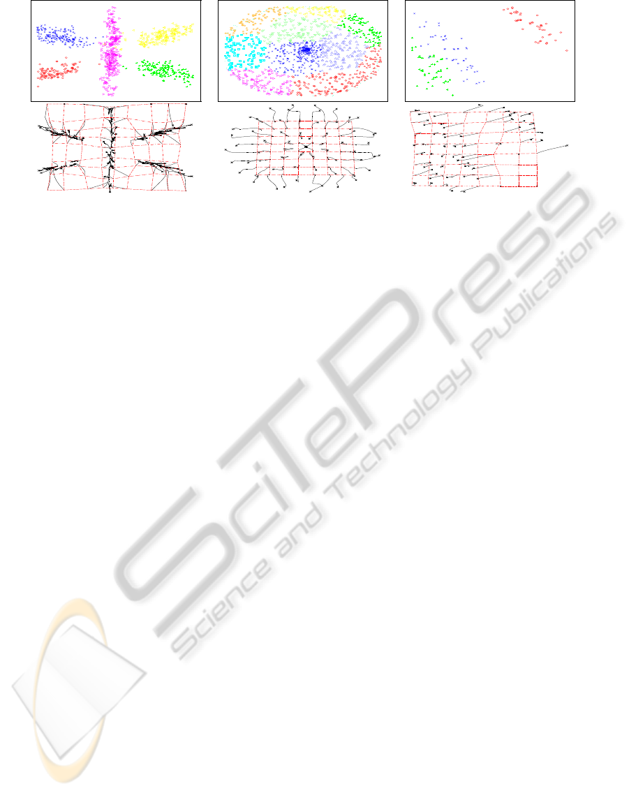
Figure 2: The results for the three datasets are given in column 1 for Art1, column 2 for Art2 and column 3 for Iris. The 1-th
row is for the map from the faGTM model. The 2-nd row is for the graphs of the g sets of curves T
k
. The mesh resulting of
the first EM step with coordinates s
(1)
k
is in red dot line.
uniform distribution on [0;0.15]. This resulting
dataset counts n = 1000 vectors with d = 15 fea-
tures.
- Art2. This dataset is a random sample from one
half of a sphere centered at origin in R
3
with ra-
dius 1, plus a circular band surrounding the 2-
th hemisphere near the great circle. This dataset
counts n = 1479 vectors of d = 3 features. The
sample from the hemisphere is clustered artifi-
cially into 10 non-overlapping classes.
- Iris. The dataset of the Iris is compound of 150
vectors in a 4-dimensional space and 3 classes.
The trajectory plot is less relevant in this situation
to reveal the 3 clusters which are less separated.
The projections for the three datasets are shown in
Figure 2. The points for the different classes have
different colors on the graphics. The results are very
encouraging, the method adds flexibility to the vec-
tors of basis function, and leads to a novel graphical
representation for the GTM.
6 CONCLUSIONS AND
PERSPECTIVE
We have proposed a hierarchical factor prior with pa-
rameters C, ρ and λ for generalizing MPPCA and
GTM. The faGTM and its prior offer several per-
spectives. For instance, the trajectory map as a com-
plement to the magnification factors (Bishop et al.,
1997; Maniyar and Nabney, 2006; Tiˇno and Giannio-
tis, 2007) can be studied further.
REFERENCES
Baek, J., McLachlan, G., and Flack, L. (2009). Mixtures
of factor analyzers with common factor loadings: ap-
plications to the clustering and visualisation of high-
dimensional data. IEEE Transactions on Pattern Anal-
ysis and Machine Intelligence.
Bishop, C., Svensen, M., and Williams, C. (1997). Mag-
nification factors for the gtm algorithm. In Fifth In-
ternational Conference on Artificial Neural Networks,
pages 64 –69.
Bishop, C. M. (1995). Neural Networks for Pattern Recog-
nition. Clarendon Press.
Bishop, C. M., Svens´en, M., and Williams, C. K. I. (1998).
Developpements of generative topographic mapping.
Neurocomputing, 21:203–224.
Dempster, A., Laird, N., and Rubin, D. (1977). Maximum-
likelihood from incomplete data via the EM algo-
rithm. J. Royal Statist. Soc. Ser. B., 39, pages 1–38.
Ghahramani, Z. and Hinton, G. E. (1996). The EM algo-
rithm for mixtures of factor analyzers. Technical Re-
port CRG-TR-96-1.
Kohonen, T. (1997). Self-organizing maps. Springer.
Maniyar, D. M. and Nabney, I. T. (2006). Visual data
mining using principled projection algorithms and in-
formation visualization techniques. In Proceedings
of the 12th ACM SIGKDD international conference
on Knowledge discovery and data mining, KDD ’06,
pages 643–648. ACM.
McLachlan, G. J. and Peel, D. (2000). Finite Mixture Mod-
els. John Wiley and Sons, New York.
Tipping, M. E. and Bishop, C. M. (1999a). Mixtures of
probabilistic principal component analyzers. Neural
Computation, 11(2):443–482.
Tipping, M. E. and Bishop, C. M. (1999b). Probabilistic
principal component analysis. Journal of the Royal
Statistical Society. Series B (Statistical Methodology),
61(3):pp. 611–622.
Tiˇno, P. and Gianniotis, N. (2007). Metric properties
of structured data visualizations through generative
probabilistic modeling. In Proceedings of the 20th in-
ternational joint conference on Artifical intelligence,
pages 1083–1088.
GENERATIVE TOPOGRAPHIC MAPPING AND FACTOR ANALYZERS
287