
MODELLING A FOREGROUND FOR BACKGROUND
SUBTRACTION FROM IMAGES
Probability Distribution of Pixel Positions based on Weighted Intensity Differences
Suil Son, Young-Woon Cha and Suk I. Yoo
School of Computer Science and Engineering, Seoul National University,
1 Kwanak-ro, Kwanak-gu, Seoul, Republic of Korea
Keywords:
Foreground detection, Foreground model, Background subtraction, Background model, Object detection.
Abstract:
To overcome a false detection problem caused by dynamic textures in background subtraction problems, a
new modelling approach is suggested. While traditional background subtraction approaches model the back-
ground, an indirect method, to detect foreground objects, the approach described here models the foreground
directly. The foreground model is given by the probability distribution of pixel positions in terms of sums
of weighted intensity differences for each pixel position between all previous images and a new image. The
combination of the weighting and the summing of the intensity differences produces a number of desirable
effects. For instance, each position in the new image which has consistently large differences will have a high
foreground probability value; each position having consistently small differences will have a low probability
value; and positions having small differences for most of the previous images but large differences for a few
of the previous images due to dynamic textures or noises will have medium probability values. The final dis-
tribution of the foreground position is computed by Kernel density estimation incorporating the neighboring
pixel differences, and foreground objects are then identified by the probability value of this distribution. The
performance of the suggested approach is then illustrated with two classes of problems and compared to other
conventional approaches.
1 INTRODUCTION
The background subtraction problem is to detect ab-
normal objects from a new image given the sequence
of its previous images. In most conventional back-
ground subtraction methods, a statistical model of the
background image, called the background model, is
formulated using the previous images and then com-
pared to the new image to detect the abnormal objects,
called the foreground. Since the background subtrac-
tion method has a wide area of application such as
tracking, identification, surveillance, and defect de-
tection, many approaches to formulating the back-
ground model have been introduced.
Wren et al.(1997) firstly proposed a background
model based on a single Gaussian over the inten-
sity value of each pixel. The single Gaussian model,
however, could not correctly represent most outdoor
scenes since small motion of objects or dynamic tex-
tures such as swaying trees or flows of water caused
the associated pixels with different intensities to be
considered as the foreground. To handle this prob-
lem, Stauffer and Grimson(1999) suggested a model
using a mixture of Gaussians. Their approach could
describe the background more accurately, but their
results sometimes deteriorated when the number of
Gaussians was selected improperly. Elgammal and
Davis(2000) proposed a non-parametric approach to
modelling the background. They adapted the kernel
density estimation (Bishop, 2006) to build the back-
ground statistics without any assumption about the
shape of the statistical model. However, when the dy-
namic textures heavily appear, their approach cause
the distribution to be a widely spread shape where
the associated pixels are detected as the foreground
regardless of their intensity values. Dalley and Grim-
son(2008) proposed a model modified from the Stauf-
fer and Grimson’s one. In this model, a set of mixture
components lying at the local spatial neighbourhood
of a pixel was suggested rather than a mixture lying at
the same pixel position. This model reduced the false
detections, but the neighbours distribution introduced
by a window caused loss of true foreground pixels.
To relax the false detection caused by dynamic
400
Son S., Cha Y. and I. Yoo S. (2012).
MODELLING A FOREGROUND FOR BACKGROUND SUBTRACTION FROM IMAGES - Probability Distribution of Pixel Positions based on Weighted
Intensity Differences.
In Proceedings of the 1st International Conference on Pattern Recognition Applications and Methods, pages 400-404
DOI: 10.5220/0003769204000404
Copyright
c
SciTePress

textures, the approaches using additional features
or formulations were proposed. Mittal and Para-
gios(2004) introduced the optical flow as the sup-
plemental feature for the background model. With
the spatial image gradient and temporal derivatives,
the approach suppressed the false detection from the
video frames of the ocean and the park with trees.
Sheikh and Shah(2005) suggested both models of a
background and a foreground. They collected fore-
ground features from the image immediately preced-
ing the current new image and used the features to
compute the probability modelling the foreground.
Since the two models by Mittal et al.(2004) and by
Sheikh et al.(2005) use features from the image right
before the current new image, it works well in those
problems like video frames where the continuity of
the sequence of images is preserved. However, its
performance gets worse as the interval between two
images in the sequence becomes larger.
In this paper, to overcome the false detection prob-
lems caused by the dynamic textures and noises, a
new approach directly modelling a foreground is sug-
gested. The proposed model is established with the
probability distribution of pixel positions in terms of
sum of weighted intensity differences between pre-
vious images and the new image. Based on this fore-
ground position model, each pixel position on the new
image having its probability value greater than the
threshold is claimed to be the one forming the fore-
ground.
2 MODELLING A FOREGROUND
2.1 Foreground Position Distribution
A foreground is defined to be a set of objects with
motion. If an object has motion, its position changes
from image to image. This means that the object’s
motion causes intensity differences of the associated
positions. Thus, for a given position if its intensity
difference between two compared images becomes
relatively large, it is more probable for that position
to be the one forming a foreground. Based on this
consideration, the probability that each position in the
new image becomes a foreground can be defined in
terms of sum of its weighted intensity differences be-
tween the new image and all the previous images.
More formally, let the number of previous images
in a sequence be N and let S be a set of pixel positions
on an image, S = {(x,y)|1 ≤ x ≤ W,1 ≤ y ≤ H, W
is a width and H is a height of an image}. Let I
j,k
for j ∈ S,k = 1,...,N, N + 1, be the intensity value of
the position j on the kth image, where the (N + 1)th
image is the new image. If L is a random variable over
all positions of pixels on the image, the probability
P
f
(L = l) that a pixel at the position l ∈ S on the new
image becomes a foreground is given by
P
f
(L = l) =
1
Z
N
∑
t=1
∑
m∈S
w(|I
l,N+1
− I
m,t
|) · δ(l,m)
(1)
where w : R → R is a weight function such that for ev-
ery x in R, w(x) = log(1 + x). The weight function is
defined to prevent the intensity difference from being
too large once it becomes large enough to be iden-
tified as a foreground. It preserves the property of
sum of original differences in identifying each posi-
tion and also gives the reasonable range of the proba-
bility used for determining the threshold of the proba-
bility to distinguish the foreground from the dynamic
textures and the background, which is explained in
section 3.
Z is a normalizing constant given by
Z =
N
∑
t=1
∑
l∈S
∑
m∈S
w(|I
l,N+1
− I
m,t
|) · δ(l,m)
(2)
where the position matching function δ returning 1
only when two matching positions are identical is
such that
δ(l, m) =
(
1 , if l = m
0 , otherwise.
(3)
2.2 Approximating Foreground Position
Distribution
In computing the probability of equation (1), it is not
easy to align two compared images exactly enough
to compute the position matching function δ(l,m).
To allow the slight misalignment, it is approximated
with the Gaussian kernel function K(l − m) (Bishop,
2006). The approximated probability
ˆ
P
f
(L = l) is
then
ˆ
P
f
(L = l) =
1
ˆ
Z
N
∑
t=1
∑
m∈S
w(|I
l,N+1
−I
m,t
|)·K(l −m) (4)
where
ˆ
Z is a normalizing constant and K is a Gaussian
kernel function. The normalizing constant
ˆ
Z is given
by
ˆ
Z =
N
∑
t=1
∑
l∈S
∑
m∈S
w(|I
l,N+1
− I
m,t
|) · K(l − m)
(5)
and the Gaussian kernel function K : R × R → R is
such that
K(l −m) =
1
2π
1
|H|
1/2
exp
−
1
2
(l −m)
T
H
−1
(l −m)
(6)
where l − m is a 2-dimensional vector and H is a 2×2
bandwidth matrix of the kernel.
MODELLING A FOREGROUND FOR BACKGROUND SUBTRACTION FROM IMAGES - Probability Distribution of
Pixel Positions based on Weighted Intensity Differences
401

(a) (b) (c) (d) (e) (f) (g)
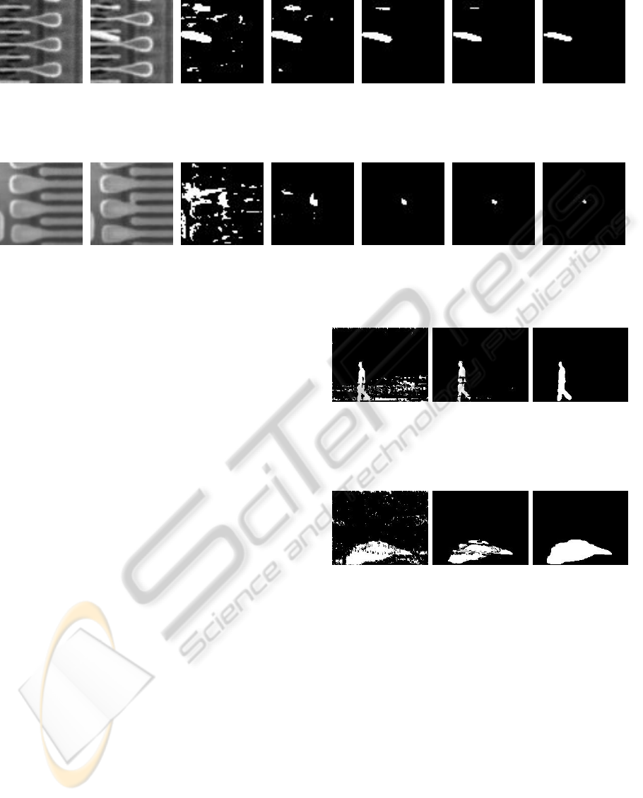
Figure 1: Background subtraction for natural scene 1. Approximated threshold by K-means algorithm: T
A
= 0.00005 (a) One
of previous images. (b) A new image. (c) T = T
A
× 0.8 (d) T = T
A
× 0.9 (e) T = T
A
× 1.0 (f) T = T
A
× 1.1 (g) T = T
A
× 1.2.
(a) (b) (c) (d) (e) (f) (g)
Figure 2: Background subtraction for natural scene 2. Approximated threshold by K-means algorithm: T
A
= 0.00005 (a) One
of previous images. (b) A new image. (c) T = T
A
× 0.8 (d) T = T
A
× 0.9 (e) T = T
A
× 1.0 (f) T = T
A
× 1.1 (g) T = T
A
× 1.2.
3 DETECTING A FOREGROUND
The probability of each position given by equation (4)
shows how probable the position becomes the fore-
ground as compared to other positions in the image.
The larger value it has, the more probable it becomes
the foreground. As mentioned in section 2.1, those
positions of some object with motion have the large
sum of intensity differences resulting in the high prob-
ability, which are thus to be considered as the fore-
ground. Those positions of objects without motion
however have the small sum of intensity differences
resulting in the low probability, considered to be as
the background. Finally those positions associated
with dynamic textures or noises have the medium
sum of intensity differences resulting in the interme-
diate probability, which should be not considered as
the foreground. To identify those positions associ-
ated with foreground, thus it is necessary to find the
boundary of probability values between foreground
and dynamic textures. Although it is not easy to find
the exact boundary in general, it may be approximated
by grouping all probability values into three groups,
high, intermediate, and low. Assuming three clusters,
the K-means algorithm (Bishop, 2006) is applied to
all probability values. The minimum value from the
cluster consisting of high values is suggested as the
approximated value of the boundary between the fore-
ground and the dynamic textures, called the threshold.
This value is then adjusted via training examples to
get the best value of threshold.
4 EXPERIMENTAL RESULTS
Our approach is applied to two classes of problems,
background subtraction from natural scenes and de-
fect detection from SEM(Scanning Electron Micro-
scope) images, with four examples. The results are
then compared to those from two conventional back-
ground subtraction approaches, one based on the ker-
nel density estimation(BS-KDE)(Ahmed Elgammal
and Davis, 2000) and the other based on the Gaussian
mixture model(BS-GMM)(Gerald Dalley and Grim-
son, 2008) with 3 × 3 windows.
4.1 Background Subtraction Problems
from Natural Scenes
The goal of the background subtraction from natural
scenes is to successfully detect the foreground objects
from the new image avoiding the false detection due
to dynamic textures. Images used for the following
two examples are assumed to contain dynamic tex-
tures.
Example 1: Given a sequence of 30 previous im-
ages including Figure 1(a), the problem is to detect
a person as the foreground from the new image of
Figure 1(b): The probability values of all the pix-
els in the image are first computed from equation (4)
using 30 previous images and the new image. The
K-means algorithm applied to those computed values
then gives the approximated threshold, T
A
= 0.00005.
Finally based on the detection results from using var-
ious values around T
A
, which are shown from Figure
1(c),(d),(e),(f), and (g), the threshold T is given to be
as same as T
A
. The result using this threshold is com-
pared to those from two other approaches in section
ICPRAM 2012 - International Conference on Pattern Recognition Applications and Methods
402
(a) (b) (c) (d) (e) (f) (g)
Figure 3: Defect detection for SEM image 1. Approximated threshold by K-means algorithm: T
A
= 0.00037 (a) One of
previous images. (b) A new image. (c) T = T
A
× 0.9 (d) T = T
A
× 1.0 (e) T = T
A
× 1.1 (f) T = T
A
× 1.2 (g) T = T
A
× 1.3.
(a) (b) (c) (d) (e) (f) (g)
Figure 4: Defect detection for SEM image 2. Approximated threshold by K-means algorithm: T
A
= 0.00005 (a) One of
previous images. (b) A new image. (c) T = T
A
× 1.0 (d) T = T
A
× 1.3 (e) T = T
A
× 1.6 (f) T = T
A
× 1.7 (g) T = T
A
× 1.8
4.3.
Example 2: Given a sequence of 30 previous im-
ages including Figure 2(a), the problem is to de-
tect a car as the foreground from the new image of
Figure 2(b): With similar procedure as in example
1, the approximated threshold T
A
is computed to be
0.00005. Based on the detection results from using
various values around T
A
, which are shown from Fig-
ure 2(c),(d),(e),(f), and (g), the threshold T is given to
be as same as T
A
. The result using this threshold is
compared to those from two other approaches in sec-
tion 4.3.
4.2 Defect Detection Problems from
SEM Images
The goal of the defect detection from SEM images
is to detect defects from the new image avoiding the
false detection due to noises and shape variations of
semiconductor’s pattern where the sequence of previ-
ous images is considered as a set of reference images.
Images used for the following two examples are as-
sumed to contain noises associated with intensity val-
ues and shape variations of semiconductor’s patterns.
Example 3: Given a sequence of 10 previous im-
ages including Figure 3(a), the problem is to detect
defects as the foreground from the new image of Fig-
ure 3(b): With similar procedure as in previous ex-
amples, the approximated threshold T
A
is given to be
0.00037. Based on the detection results from using
various values around T
A
, which are shown from Fig-
ure 3(c),(d),(e),(f), and (g), the threshold T is given
to be T = T
A
× 1.3 = 0.00048. The result using this
threshold is compared to those from two other ap-
(a) (b) (c)
Figure 5: Comparison of background subtraction results for
natural scene 1. (a) Result from BS-KDE. (b) Result from
BS-GMM. (c) Result from our foreground model.
(a) (b) (c)
Figure 6: Comparison of background subtraction results for
natural scene 2. (a) Result from BS-KDE. (b) Result from
BS-GMM. (c) Result from our foreground model.
proaches in section 4.3.
Example 4: Given a sequence of 5 previous im-
ages including Figure 4(a), the problem is to detect
defects as the foreground from the new image of Fig-
ure 4(b): With similar procedure as in previous ex-
amples, the approximated threshold T
A
is given to be
0.00030. Based on the detection results from using
various values around T
A
, which are shown from Fig-
ure 4(c),(d),(e),(f), and (g), the threshold T is given
to be T = T
A
× 1.6 = 0.00048. The result using this
threshold is compared to those from two other ap-
proaches in section 4.3.
MODELLING A FOREGROUND FOR BACKGROUND SUBTRACTION FROM IMAGES - Probability Distribution of
Pixel Positions based on Weighted Intensity Differences
403

(a) (b) (c)
Figure 7: Comparison of defect detection results for SEM
image 1. (a) Result from BS-KDE. (b) Result from BS-
GMM. (c) Result from our foreground model.
(a) (b) (c)
Figure 8: Comparison of defect detection results for SEM
image 2. (a) Result from BS-KDE. (b) Result from BS-
GMM. (c) Result from our foreground model.
4.3 Comparison to Other Approaches
For each of four examples in section 4.1 and 4.2, our
approach is compared to two other approaches, the
kernel density estimation (BS-KDE) (Ahmed Elgam-
mal and Davis, 2000) and the Gaussian mixture model
with 3 × 3 windows (BS-GMM) (Gerald Dalley and
Grimson, 2008). Figure 5, 6, 7, and 8 shows results
from using three approaches.
For the first two examples of the background sub-
traction problem, as shown in Figure 5 and 6, our ap-
proach results in clearly described objects of a per-
son and a car. The results from two other approaches
however describe not clear and noisy objects due to
dynamic textures.
For the next two examples of the defect detection
problem, as shown in Figure 7 and 8, our approach
detects defects only but two other approaches of the
BS-KDE and the BS-GMM detects defects and also
other defect-free areas as defects.
5 CONCLUSIONS
A new approach using a foreground model was sug-
gested for solving the background subtraction prob-
lem and the related defect detection problem. The
foreground model has been formulated using the
weighted intensity differences between a new image
and all previous images. The suggested approach has
relaxed the difficulty of detecting the foreground from
the images containing dynamic textures and noises, as
compared to the traditional approaches using a back-
ground model.
ACKNOWLEDGEMENTS
The ICT at Seoul National University provided re-
search facilities for this study, and this work was also
supported by the Brain Korea 21 Project in 2011.
REFERENCES
Ahmed Elgammal, D. H. and Davis, L. (2000). Non-
parametric model for background subtraction. In Eu-
ropean Conference on Computer Vision.
Bishop, C. M. (2006). Pattern recognition and machine
learning. Springer, 1st edition.
Gerald Dalley, J. M. and Grimson, W. E. L. (2008). Back-
ground subtraction for temporally irregular dynamic
textures. In IEEE Workshop on Applications of Com-
puter Vision.
ICPRAM 2012 - International Conference on Pattern Recognition Applications and Methods
404
