
EXTRACTION OF BLOOD DROPLET FLIGHT TRAJECTORIES
FROM VIDEOS FOR FORENSIC ANALYSIS
L. A. Zarrabeitia, D. A. Aruliah and F. Z. Qureshi
Faculty of Science, University of Ontario Institute of Technology, Oshawa, ON, Canada
Keywords:
Stereo reconstruction, Tracking, Droplets, Blood flight, Multi-target tracking.
Abstract:
We present a method for extracting three-dimensional flight trajectories of liquid droplets from video data.
A high-speed stereo camera pair records videos of experimental reconstructions of projectile impacts and
ensuing droplet scattering. After background removal and segmentation of individual droplets in each video
frame, we introduce a model-based matching technique to accumulate image paths for individual droplets. Our
motion detection algorithm is designed to deal gracefully with the lack of feature points, with the similarity of
droplets in shape, size, and color, and with incomplete droplet paths due to noise, occlusions, etc. The final
reconstruction algorithm pairs two-dimensional paths accumulated from each of the two cameras’ videos to
reconstruct trajectories in three dimensions. The reconstructed droplet trajectories constitute a starting point
for a physically accurate model of blood droplet flight for forensic bloodstain pattern analysis.
1 INTRODUCTION
Bloodstain pattern analysis (BPA) comprises tech-
niques for inferring spatial locations of bloodletting
events from bloodstains found at crime scenes (Bevel
and Gardner, 2008; Buck et al., 2011). At present,
BPA, to a large extent, is a qualitative sub-discipline
of forensic science. Our present goal is to im-
prove computational models for bloodletting events
and bloodstain pattern formation. These models, we
believe, will be of immense value to forensic inves-
tigators and BPA specialists for reasoning accurately
from images of bloodstain patterns at crime scenes.
Furthermore, such models are required to develop the
next generation of BPA software for inference and as-
sessing uncertainties in BPA.
Stringing (Buck et al., 2011) is a common method
for locating the bloodletting event responsible for a
particular bloodstain pattern. This method relies on
the assumption that blood droplets move in straight
lines, ignoring the effects of gravity and aerodynamic
drag. Stringing can provide reasonable approximate
locations projected onto a horizontal plane. At short
distances, stringing may also provide estimates for the
height of the bloodletting event. More accurate bal-
listic models that incorporate viscous drag forces and
gravity, are only used when the stringing method pro-
duces unreasonable locations or speeds (Buck et al.,
2011). Our results suggest that the effects of gravity
and drag are noticeable, even over the short distances
and time scales recorded in our experiments.
The present work is concerned with reconstruct-
ing 3D trajectories of blood droplets from high-speed
video data. We have developed a stereo vision sys-
tem capable of tracking individual blood droplets in
high-speed videos (1300 frames per second) and auto-
matically reconstructing their three-dimensional (3D)
flight trajectories. In each experiment, the stereo cam-
era pair captures a high-speed video of the impact of a
BB pellet with a ballistic gel encasing transfer blood
(i.e., approximating human flesh); this scenario is in-
tended to simulate a penetrating trauma (e.g., a gun-
shot wound). Upon impact, the ballistic gel is punc-
tured and expels its contents at high speeds. Blood
droplets then fly through the air hitting nearby sur-
faces to create bloodstain patterns. Our video record-
ings of these simulated bloddletting events allow us
to study the effects of gravity and aerodynamic drag
on blood droplet trajectories (see Figure 1). We also
photograph the resulting bloodstain patterns.
Estimation of individual blood droplet trajectories
from recorded videos comprises three stages:
1. subtracting the background and connected-
component analysis to identify images of
individual blood droplets in each video frame;
2. tracking of individual blood droplets between
video frames to generate 2D droplet in each cam-
era’s view; and
3. estimating three-dimensional trajectories by link-
142
A. Zarrabeitia L., A. Aruliah D. and Z. Qureshi F. (2012).
EXTRACTION OF BLOOD DROPLET FLIGHT TRAJECTORIES FROM VIDEOS FOR FORENSIC ANALYSIS.
In Proceedings of the 1st International Conference on Pattern Recognition Applications and Methods, pages 142-153
DOI: 10.5220/0003770201420153
Copyright
c
SciTePress

(a) (b) (c)
Figure 1: (a) BB pellet impacting ballistic gel containing transfer blood. (b) Tracking individual blood droplets in high-speed
video (1300 frames per second). (c) Reconstructed blood droplet trajectories. Notice the effects of gravity and viscous drag
forces even for short trajectories.
ing image paths from each camera’s view.
We present a model-based approach to tackle this
challenging problem.
The long-term goal that motivates the present
study is to develop accurate physics-based models of
blood flight to reconstruct impact conditions in blood-
stain pattern analysis. As a first step, then, we record
and compare flight patterns with models traditionally
used in this field. Thus, we automate the extraction
and synthesis of 3D trajectories of individual droplets
from video recordings.
1.1 Related Work
While object-tracking has been studied extensively
within the computer vision community (see, e.g.,
(Yilmaz et al., 2006)), tracking flight paths of liq-
uid droplets across a large number of frames of video
presents considerable challenges. In particular, track-
ing individual blood droplets involves identifying
hundreds of semi-transparent, quasi-deformable ob-
jects of very similar sizes and appearances. Tracking
can be formulated by establishing correspondences
between detected objects represented by points (or
targets) across frames. Point correspondence is a
complicated problem, especially in the presence of
occlusions, misdetections, and objects entering or
leaving the field of view. The most obvious diffi-
culty in our problem arises from the similarity be-
tween blood droplets; tracking techniques based on
detection of feature points (such as in (Yilmaz et al.,
2006)) are not effective in this context. We apply
an approach similar to that followed in (Balch et al.,
2001) to detect individual blood droplets in each of
the video frames captured by each camera. The prob-
lem in this earlier work is similar to ours, albeit with
fewer targets and greater information in each frame.
A core requirement of tracking algorithms is solv-
ing assignment problems to match objects between
successive video frames. The Kuhn-Munkres Al-
gorithm (also known as the Hungarian algorithm
(Kuhn, 1955; Munkres, 1957)) was proposed in the
mid-1950s to solve linear assignment problems in
polynomial time. Bourgeois and Lassalle extended
the Kuhn-Muhnkres algorithm to handle rectangular
problems in 1971 (Bourgeois and Lassalle, 1971). A
more recent effort, in addressing the sailor assign-
ment problem, produced a variant of the rectangu-
lar method for sparse graphs and multiobjective prob-
lems (Dasgupta et al., 2008). For more recent surveys
of rectangular assignment problems in the context of
multiple target tracking and in general, see (Poore
and Gadaleta, 2006) and (Bijsterbosch and Volgenant,
2010).
Among algorithms proposed to solve the problem
of multi-target tracking are MHT (Reid, 1979) and
Greedy Optimal Assignment (Veenman et al., 2001).
The latter is used in (Betke et al., 2007) to track a large
number of bats. A similar strategy is used in (Balch
et al., 2001) for tracking the behaviour of live insects.
In (Khan et al., 2003) and (Khan et al., 2005a), the au-
thors propose a particle filter for tracking the motion
of insects. Both of these studies involve applying a
Markov field to model insect interactions and assum-
ing that the targets actively avoid collisions. (Khan
et al., 2005b) extends these works to deal with split
and merged measurements. A problem similar to ours
is studied in (Grover et al., 2008) and (Straw et al.,
2011). They succeed in reconstructing the 3D trajec-
tories of multiple targets — in these instances, flies
— from a multi-camera setup. The movements of in-
sects are arguably harder to predict than the ballistic
trajectory of blood droplets. On the other hand, the
insect-tracking problem is less sensitive to errors in
prediction as there are fewer targets moving at lower
speeds and the number of targets does not change (as
compared to flying droplets that can split and merge).
2 BACKGROUND REMOVAL AND
SEGMENTATION
The cameras detect minute lighting fluctuations be-
EXTRACTION OF BLOOD DROPLET FLIGHT TRAJECTORIES FROM VIDEOS FOR FORENSIC ANALYSIS
143
tween frames due to the high frame-rate even under
carefully controlled conditions. As such, we employ
a dynamic background model (Balch et al., 2001) to
identify pixels corresponding to blood droplets. Once
the background is subtracted, a binary mask is super-
imposed to identify target clusters of pixels that os-
tensibly correspond to fluid droplets.
2.1 Identifying the Background
Our proposed dynamic background model success-
fully compensates for noticeable fluctuations in over-
all image intensity between successive frames. Let
I
(k)
denote the image intensity in the k
th
video frame
and let B
(k)
denote the corresponding background
model. Both and I
(k)
and B
(k)
are matrices with real-
valued entries between 0.0 and 1.0. We also con-
struct the corresponding binary mask F
(k)
(i.e., a ma-
trix with 0-or-1 entries) to indicate pixels in frame k
associated with blood droplets (see Figure 2).
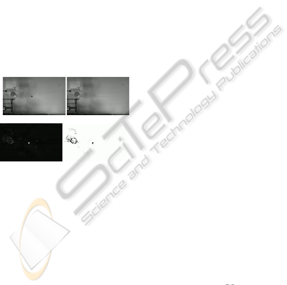
(a) (b)
(c) (d)
Figure 2: Blood droplet segmentation: (a) Original image
intensity I
(k)
. (b) Background model B
(k)
. (c) Deviation
from the background model
I
(k)
− B
(k)
. (d) Foreground
mask F
(k)
.
The aforementioned lighting fluctuations preclude
using a constant background model B
(k)
= B
(0)
= I
(0)
in all frames. Instead, we apply the dynamic linear
model
B
(0)
= I
(0)
, (1a)
B
(k+1)
= (1 − α)B
(k)
+ αI
(k)
, α ∈ [0,1]. (1b)
The coefficient α in (1b) controls how quickly the
background model adapts to the changes in the back-
ground (e.g., newly formed bloodstains on the back
wall). Small values of α imply a slow learning speed.
For example, when α = 0, the result is a constant
background model; such a model is incapable of deal-
ing with changes in illumination or in the background.
Conversely, large values of α may cause the moving
droplets to be considered part of the background; this
leads to a ghosting effect where droplets are detected
twice in each frame. More sophisticated techniques
(e.g., random Markov fields) could alternatively be
used for background subtraction; however, in this ap-
plication context, such models unnecessarily intro-
duce additional complexity without significant gain.
Having determined the background model B
(k)
in
the k
th
frame, the binary mask F
(k)
is computed pixel-
wise by the rule
F
(k)
(u,v) =
(
1 if
I
(k)
(u,v)− B
(k)
(u,v)
> ε
bg
,
0 otherwise.
(2)
The preselected threshold value ε
bg
∈ [0,1] in (2) has
to be chosen carefully. The challenge is to ensure cap-
turing droplets flying over darker regions of the back-
ground, while ignoring intensity fluctuations between
frames.
Suitable values of α and ε
bg
cannot generally be
determined a priori; they depend on ambient exper-
imental conditions indiscernible by the naked eye.
This problem can be alleviated, but not completely
solved, by previewing a few frames taken at high
speed prior to the experiment. Previewing a few
frames allows us to relocate the lights to maximize
contrast and reduce shadows.
2.2 Segmentation of Individual Droplets
The process of background removal yields a sequence
of binary masks
n
F
(k)
o
N
frames
k=0
. From the binary mask
F
(k)
of the k
th
video frame, the clusters of pixels in the
connected components of F
(k)
correspond to individ-
ual foreground objects. Some of these clusters corre-
spond to genuine blood droplets, but some others are
false positives (e.g., the projectile, falling gelatin, and
noise or illumination artifacts). False positives are fil-
tered out by discarding clusters that are either too big
or too small. We refer to the pixel clusters associated
with blood droplets as targets and we denote the set
of all targets accepted in frame k by T
(k)
.
Each target t ∈ T
(k)
has a number of properties
that are recorded. For instance, the target t has an area
a (in pixels) and associated raw moments M
00
, M
01
,
and M
10
(see, e.g., the documentation of OPENCV
(Bradski, 2000) for appropriate definitions). The mo-
ments of t are required to compute the image coordi-
nates of the target’s centroid (u,v) which is consid-
ered the location of the blood droplet associated with
the target. These properties are recorded for each tar-
get in each frame and are used to match targets in suc-
cessive frames for motion tracking.
ICPRAM 2012 - International Conference on Pattern Recognition Applications and Methods
144

3 TRACKING TARGET PATHS IN
IMAGES
Tracking the motion of an object using video data en-
tails identifying images of the same points (targets)
in a sequence of successive frames. When dealing
with small numbers of easily distinguishable rigid ob-
jects (e.g., when colour and shape are clearly distinct
or when obvious feature points are available), associ-
ating targets from frame to frame is straightforward.
However, when trying to track large collections of
very similar objects, more sophisticated measures are
needed to assess the credibility of the reconstructed
motion of individual targets.
3.1 Limitations of Tracking Targets
Strictly Frame-by-frame
To state the tracking problem in concrete terms, re-
call that T
(k)
denotes the set of all targets (images of
droplets) detected in frame k. Each target in t
(k)
∈
T
(k)
can be thought of as a pair t
(k)
=
u
(k)
,v
(k)
of pixel coordinates (given by the target’s centre of
mass). Targets have additional properties other than
their centroids (e.g., areas, moments, etc.) that can be
used in tracking. Many tracking algorithms (e.g., in
(Balch et al., 2001)) are based on linking targets in
T
(k)
(i.e., from frame k) directly to targets in T
(k+1)
(i.e., from frame k + 1).
Such approaches work well when the cardinality
of the target sets does not vary significantly between
frames. For the droplet tracking problem, this as-
sumption breaks down in a number of ways:
1. a false target t
(k)
is spuriously detected in frame
k, i.e., pixels contaminated by noise are mistaken
for a legitimate physical object in the scene;
2. a true target t
(k)
is not detected by the camera in
frame k + 1;
3. a true target t
(k)
is temporarily occluded by an-
other object in frame k + 1;
4. a target t
(k)
temporarily leaves the field of view
between frames k and k + 1;
5. a target t
(k+1)
returns to the field of view between
frames k and k + 1;
6. a target t
(k)
permanently leaves the field of view
between frames k and k + 1; and
7. a target t
(k+1)
initially enters the field of view be-
tween frames k and k + 1.
These modes of failure are the norm rather than ex-
ceptions. In case (1), it is necessary to handle spuri-
ous detections gracefully. The cases (2), (3), and (4)
are temporary failures; it is best not to match the tar-
get t
(k)
∈ T
(k)
with any target in T
(k+1)
. Similarly,
in case (5) when the target t
(k+1)
is detected again in
frame k + 1, it should be paired with a candidate from
a frame prior to frame k (i.e., the most recent frame
in which the corresponding droplet was detected). Fi-
nally, the situations (6) and (7) should be considered
only when there is no suitable candidate target in any
later or earlier frames respectively.
3.2 Assignment Problems for Tracking
We modify the formulation of the tracking problem
to allow for the difficulties outlined in Section 3.1.
The key problem that needs to be solved at each stage
is an assignment problem. Assignment or matching
problems constitute a fundamental class of problems
in combinatorial optimization. In specific language,
let A and B be finite sets (i.e., vertices of a bipartite
graph), let cost : A×B → R be a cost function associ-
ated edges between A and B, and let M ⊂ P (A × B)
be a proper subset of the power set P (A × B). The
Assignment Problem (AP) is to construct a matching
M ⊂ A × B such that the total cost summed over all
edges in M is minimized, i.e.,
min
M∈M
∑
(a,b)∈M
cost(a,b). (3)
If
|
A
|
=
|
B
|
are equal and M consists of all pos-
sible matchings that cover both A and B, the problem
(AP) is called a Linear Assignment Problem (LAP). If
|
A
|
6=
|
B
|
, and M consists of all matchings that cover
the smaller set, the problem (AP) is called a Rectan-
gular Linear Assignment Problem (RLAP). Observe
that the constraint M on the set of possible match-
ings is necessary; otherwise, for many cases, the min-
imizer would simply be the empty matching M =
/
0.
Assuming for the moment that the constraint M ⊂
P (A × B) is known, we shall assume henceforth that
“M = SolveAP(A,B,cost, M )” (4)
means “Solve (AP) by computing the matching
M ∈ M that minimizes the sum in (3).” We implicitly
assume that a solution of (AP) exists as does a rea-
sonable algorithm for computing it. For all practical
purposes, we use the techniques in (Dasgupta et al.,
2008) to compute M in (4).
In some cases of (AP), not all edges are present
in the bipartite graph, i.e., some of the elements of
A are not connected to elements of B. This as-
signment problem can still be solved using a variant
of the Kuhn-Munkres algorithm that assigns (prac-
tically) infinite cost to absent edges (see (Dasgupta
et al., 2008)). The missing edges also introduce the
constraint M ⊂ P (A × B).
EXTRACTION OF BLOOD DROPLET FLIGHT TRAJECTORIES FROM VIDEOS FOR FORENSIC ANALYSIS
145

As an example of an assignment problem in track-
ing, the approach followed by (Balch et al., 2001) is
to find, at step k, a matching
M
(k)
= SolveAP(T
(k)
,T
(k+1)
,dist,M ), (5)
where M consists of all matchings that cover either
T
(k)
or T
(k+1)
and
dist
t
(k)
,t
(k+1)
=
t
(k)
− t
(k+1)
2
2
. (6)
There is no problem computing the cost for any edge
since it is merely the Euclidean distance.
In our formulation, we solve an assignment prob-
lem (3) where “A” is a set of paths and “B” are tar-
gets (rather than targets and targets as in (Balch et al.,
2001)). To the best of our knowledge, this formula-
tion differs from previous tracking work that matches
targets strictly between subsequent frames. Specifi-
cally, a path is an ordered list of one or more targets
[t
(k
1
)
,t
(k
2
)
,...,t
(k
s
)
] occurring in a strictly increasing
sequence of frames (i.e., so that k
1
< k
2
< ·· · < k
s
).
Notice that we do not require that successive targets
in a given path occur in successive video frames (i.e.,
that t
(k)
∈ T
(k)
absolutely must be followed by some
t
(k+1)
∈ T
(k+1)
) as we wish to deal with situations
enumerated in Section 3.1 gracefully. With this ter-
minology, we consider a set P
(k)
of paths linking tar-
gets in a strictly increasing subsequence drawn from
the 0
th
frame up to and including the k
th
frame.
Our multi-target tracking problem can then be ex-
pressed recursively using the solution of an assign-
ment problem at each step. In particular, the desired
matching is
M
(k)
= SolveAP(P
(k)
,T
(k+1)
,
d
dist,
c
M ), (7)
where
d
dist is defined using a path-based predictive
model described in Section 3.3. The set
c
M is a lit-
tle harder to describe; it consists of matchings M with
the property that, if
d
dist(p,t) < ∞, then M covers at
least one of p or t (but not necessarily both).
3.3 A Model-based Distance Metric
We do not solve the assignment problem by minimiz-
ing a sum of Euclidean distances between targets in
successive frames as in (6). Instead, we track tar-
get motion by minimizing the distances between tar-
gets in the next frame and targets predicted using the
paths. Predictive algorithms usually include a step
in which a model for each target’s motion is learned
(e.g., by a Bayesian network (Nillius et al., 2006) or a
Kalman Filter (Iwase and Saito, 2004)). In the present
context, we exploit basic models of droplet motion.
Projectiles follow simple parabolic trajectories
(with constant horizontal speeds and constant vertical
acceleration g ' 9.81ms
−2
) in the absence of aerody-
namic drag forces. The projection of such ballistic
trajectories in the image plane are similarly quadratic
curves. Even accounting for viscous drag effects,
over sufficiently short time intervals (as is the case
for high-speed video), quadratic polynomials provide
robust approximations.
Thus, given a path p ∈ P
(k)
corresponding to some
droplet’s partial motion up to and including frame k,
the estimated image coordinates of the target in frame
k + 1 are given by
ˆ
t
(k+1)
p
=
ˆu
(k+1)
p
ˆv
(k+1)
p
!
=
a
u
τ
2
k+1
+ b
u
τ
k+1
+ c
u
a
v
τ
2
k+1
+ b
v
τ
k+1
+ c
v
, (8)
where τ
k+1
is the time corresponding to frame k + 1.
The coefficients a
u
, a
v
, b
u
, b
v
, c
u
, and c
v
are deter-
mined using standard polynomial least-squares fitting
based on the targets in the path p. In the first few
frames, if a least-squares quadratic cannot be used to
fit targets in path p, polynomials of degree 0 or 1 are
generated to predict
ˆ
t
(k+1)
p
instead.
Given a path p ∈ P
(k)
, the predicted target
ˆ
t
(k+1)
p
from (8) is used to define the modified cost function
d
dist in (7) for match p to targets in T
(k+1)
. To evaluate
a proposed matching M
(k)
⊆ P
(k)
× T
(k+1)
, the cost
function is given by
d
dist
p,t
(k+1)
=
t
(k+1)
−
ˆ
t
(k+1)
p
2
2
. (9)
That is, when comparing different assignments of
paths p ∈ P
(k)
to candidate targets t
(k+1)
∈ T
(k+1)
, this
cost function penalizes targets that deviate too much
(in Euclidean distance) from the prediction
ˆ
t
(k+1)
p
.
3.4 A Predictive Tracking Algorithm
With an explicit specification of the prediction strat-
egy (8) and the cost function (9), we can now provide
a high-level description of our approach to tracking
targets through the video data in Algorithm 1.
Observe that, rather than keeping track of in-
dividual collections of paths P
(k)
, all the paths are
simply accumulated into a single set. The loop at
line 4 accumulates a set of candidate matches for p
in S; corresponding edges are added to E
(k)
in line 7.
The purpose of accumulating E
(k)
is for various
performance enhancements exploiting sparsity for
solving (7) for the matching M
(k)
at line 8 (as in
(Dasgupta et al., 2008)). The final loop at line 9
extends the paths p covered by M
(k)
once the matched
targets t
(k+1)
∈ T
(k+1)
have been determined. Finally,
ICPRAM 2012 - International Conference on Pattern Recognition Applications and Methods
146

Algorithm 1: Tracking and assembling image paths.
Input: Set of targets in each frame {T
(k)
}
N
frames
k=0
Output: Set P of (possibly incomplete) paths
1: P ←
[t
(0)
] | t
(0)
∈ T
(0)
{singleton lists}
2: for k = 0 : N
frames
− 1 do
3: E
(k)
←
/
0
4: for each path p ∈ P do
5: Predict
ˆ
t
(k+1)
p
from p using (8)
6: Find S ⊆ T
(k+1)
within ε
track
of
ˆ
t
(k+1)
p
7: E
(k)
← E
(k)
∪ {(p,t
(k+1)
) | t
(k+1)
∈ S }
8: M
(k)
= SolveAP(P
(k)
,T
(k+1)
,
d
dist,
c
M ) with
M as in (7) and
d
dist as in (9)
9: for each edge (p, t
(k+1)
) ∈ M
(k)
do
10: Replace p ∈ P by p with t
(k+1)
appended
11: Remove t
(k+1)
from T
(k+1)
12: P ← P ∪ {[t
(k)
] | t
(k)
∈ T
(k)
}
at line 12, the set of paths P is extended with new
paths containing singleton paths
h
t
(k+1)
i
of targets in
T
(k+1)
not covered by M
(k)
.
4 RECONSTRUCTION OF 3D
TRAJECTORIES
Each camera in our studies accumulates a collection
of paths in image coordinates as outlined in Section 3.
The problem, then, is to match image paths captured
by each camera to produce three-dimensional trajec-
tories. For convenience, we refer to the two cameras
as Camera I and Camera II and we refer to the asso-
ciated sets of image paths produced by Algorithm 1
as P
I
and P
II
respectively. The cameras are calibrated
so that their intrinsic and extrinsic parameters, includ-
ing the location and orientation of Camera II relative
to Camera I, are known. The calibration process is
discussed in section 5.1. We sketch the essential pro-
cedure in Algorithm 2 and fill in the details in Sec-
tions 4.1 and 4.2.
The result of Algorithm 2 is a set C of curved tra-
jectories consisting of three-dimensional world coor-
dinates of points. Actually, since each point on the
trajectory is matched to a particular video frame k,
we store the image frame k and a measure of error
d
(k)
with the world coordinates r
(k)
of each point in
the computed trajectory.
4.1 Reconstructing World Coordinates
Given a pixel (u
I
,v
I
) in image coordinates captured
by Camera I, it is straightforward to determine a line
Algorithm 2: Reconstructing trajectories in 3D.
Input: Collections of image paths P
I
and P
II
captured
by Camera I and Camera II respectively
Output: Set C of trajectories in three dimensions
1: C ←
/
0
2: for p
I
∈ P
I
do
3: for p
II
∈ P
II
do
4: K ← set of common frames of p
I
and p
II
5: if
|
K
|
> K
min
then
6: c ←
/
0
7: for k ∈ K do
8: Select t
(k)
I
from p
I
, t
(k)
II
from p
II
9: Back-project t
(k)
I
onto line `
(k)
I
10: Back-project t
(k)
II
onto line `
(k)
II
11: Find distance d
(k)
between `
(k)
I
& `
(k)
II
12: Find midpoint r
(k)
∈ R
3
13: Append tuple (k, r
(k)
,d
(k)
) onto c
14: C ← C ∪{c}
15: Define dist(p
I
, p
II
) =average of d
(k)
16: M = SolveAP(P
I
,P
II
,dist,M ) with
M as in (7) and dist as above
`
I
⊆ R
3
for which every point in the line is projected
onto the pixel (u
I
,v
I
) by Camera I. The details re-
quired to compute a representation of `
I
involve ho-
mogeneous coordinates and Camera I’s intrinsic and
extrinsic parameters; see, e.g., (Hartley and Zisser-
man, 2004) for more details. The computation is iden-
tical for Camera II, so, lines 9 and 10 of Algorithm 2
simply refer to this procedure as “back-projecting”
the pixels t
(k)
I
and t
(k)
II
onto the spatial lines `
(k)
I
and
`
(k)
II
respectively.
Given representations of the lines `
(k)
I
and `
(k)
II
, it is
elementary to find the shortest distance d
(k)
between
the two lines. We refer to the world coordinates of the
midpoint of the corresponding line segment between
the two closest points on either line as r
(k)
. Presum-
ably, if two back-projected lines actually intersect, the
computed error d
(k)
would be zero; as such, the dis-
tance d
(k)
is a reasonable proxy for the error in using
r
(k)
as the supposed spatial point that corresponds to
image points t
(k)
I
and t
(k)
II
simultaneously.
The tentative curves in world coordinates are ac-
cumulated in line 13 of Algorithm 2. These curves
consist of the midpoints r
(k)
as described above. The
frame coordinate k and the length d
(k)
are stored also
(the latter providing a measure of pointwise error).
4.2 Matching Image Paths to Space
Curves
After the space curves are built up in Algorithm 2, it
EXTRACTION OF BLOOD DROPLET FLIGHT TRAJECTORIES FROM VIDEOS FOR FORENSIC ANALYSIS
147

remains to figure out which paths in P
I
and P
II
actu-
ally do correspond to a physically reasonable curve c
in 3D. The construction of a distance function dist at
line 15 can be used to set up another assignment prob-
lem. The function dist(p
I
, p
II
) computes the average
value d
(k)
, i.e.,
d =
1
|
K
|
∑
k∈K
d
(k)
, (10)
where K is the set of common frames of p
I
and p
II
.
For paths p
I
and p
II
deemed obviously incompatible,
dist(p
I
, p
II
) = ∞.
The metric defined in (10) allows us to solve an-
other final assignment problem to figure find a match-
ing of paths from either camera (and hence the desired
three-dimensional trajectories). Again, rather than as-
sume that one of the sets P
I
or P
II
must be covered,
the set M ⊂ P (P
I
× P
II
) has a more subtle definition.
Any matching M ∈ M has the property that, for any
edges (p
I
, p
II
) such that dist(p
I
, p
II
) < ∞, one of p
I
or
p
II
is covered by M (as in (7)).
5 EXPERMIENTS AND ANALYSIS
Our experimental apparatus consists of two video
cameras because real-world coordinates of the flight
paths cannot be obtained by a single camera. How-
ever, the two-dimensional images provided by a sin-
gle camera still provide useful qualitative informa-
tion. For instance, it is plainly visible that grav-
ity plays an important role in blood droplets’ curved
trajectories even at small distances. This observa-
tion brings into question the validity of the string-
ing method for inferring the location of the blood-
letting event. Furthermore, we can later combine
the two-dimensional information from both cameras
to build accurate three-dimensional trajectories with
real-world measurements.
5.1 Experimental Setup
Figure 3 shows our experimental setup. The exper-
iments are set up on a steel table with dimensions
roughly 0.9 × 3.0 m. Plywood boards with a white
vinyl finish are placed along the two edges opposite
to the stereo camera pair. These boards act as walls
to contain the splatter and to provide a uniform back-
ground for the experiments
1
. The target is a thin latex
packet containing 20 ml of transfer blood encased in
1
Different surfaces can be clamped onto the walls to
study blood-surface interaction responsible for bloodstain
pattern formation. We plan to study this issue in the future.
Figure 3: Experimental setup showing ballistic gel contain-
ing transfer blood. Experiments are captured using a stereo
camera pair capable of recording high-speed video.
gelatin designed to approximate human flesh. The tar-
get is raised off the table with a lab jack. The paintball
gun sits directly behind the target.
Two high-speed cameras, protected by sheets of
Plexiglas, record the experimental setup from two
viewpoints, capturing videos necessary to reconstruct
the blood droplets’ trajectories in 3D. In the follow-
ing discussion, we will refer to them as the frontal
and lateral cameras, in reference to their position
around the experiment table. Fourteen 500 W work
lights illuminate the scene, allowing cameras to cap-
ture videos at 1300 frames per second. A triggering
mechanism controls the two cameras to capture syn-
chronized videos. Each experiment begins by record-
ing the calibration rig—a flat checkerboard pattern—
moving through the cameras’ fields of view. These
calibration videos are used to compute each individ-
ual cameras’ intrinsic and extrinsic parameters (Hart-
ley and Zisserman, 2004). Once calibrated, the cam-
eras are configured to record the experimental area at
high speed and the gun is fired. Upon impact with
the target, the latex container breaks, causing the gel
and the liquid to escape and leaving “bloodstains”
on the wall. The process typically takes anywhere
from 0.6 to 1.3 seconds, producing up to 1690 grey-
scale frames from each camera. Video resolution is
1280 × 800 pixels.
Our system has a very low threshold for errors,
so we devised the following calibration scheme. We
point a laser at the scene and record a pair of videos
showing the laser dot moving through the scene. The
position of the laser dot in each video frame can then
be used to verify the camera pair calibration (see Fig-
ure 4). A modified version of the segmentation proce-
dure from Section 2.2 is used to detect the laser dot;
only the brightest region is kept if the segmentation
finds more than one connected component. We as-
sume that the location and direction of the cameras
do not change during the course of the experiment,
i.e, that the extrinsic parameters computed during the
calibration process do not change. The laser verifica-
ICPRAM 2012 - International Conference on Pattern Recognition Applications and Methods
148
tion procedure described above is repeated after each
experiment to validate the preceding assumption.
A failure in the second laser verification signals
that at least one of the cameras moved during the ex-
periment, This could happen due to kinetic energy be-
ing transferred to the walls or the camera base by re-
coil from the gun or the bullet bouncing off the walls.
In either case, the experiment is discarded as we can-
not use visual cues from the experiment table to com-
pensate for this movement.
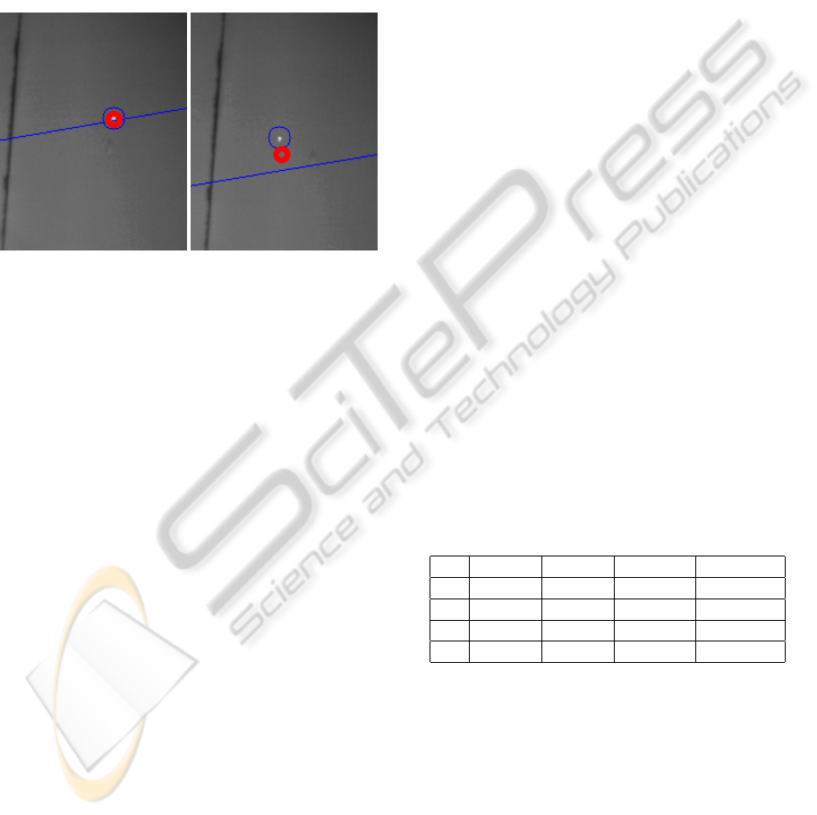
Figure 4: Calibration verification by shining a laser at the
observed region. In these figures, thin blue circles depict the
laser dot, blue lines represent the epipolar line correspond-
ing to the the laser dot in the other camera, and the thick
red circles show the re-projection of the 3D reconstruction
of the laser dot. The left image shows a successful calibra-
tion. Here, the epipolar line crosses the laser dot and the
re-projection coincides with the original location. The right
image shows an inaccurate calibration. One of the cameras
has moved, perhaps due to the vibrations generated by the
recoil of the gun.
A few pictures of the bloodstains are captured be-
fore cleaning up the lab and preparing for the next
experiment. These pictures are taken using similar
equipment and techniques available to a forensic in-
vestigator capturing photographic evidence of blood-
stains at a crime scene. 48 successful experiments
were conducted.
5.2 Validation by Visual Inspection
A single video from an experiment yields hundreds
of image paths from each camera. It is infeasible to
track more than a few trajectories manually, far fewer
than would required to obtain a statistically represen-
tative sample of the entire set of trajectories. Fur-
thermore, correlating trajectories tracked by hand to
ones tracked automatically by our system would re-
quire a scheme to account for quantitative differences
between clusters of pixels identified subjectively by
a human operator versus those segmented automati-
cally by the scheme outlined in Section 2.2. Thus, we
need a way to allow the operator to quickly track and
compare hundreds of tracks simultaneously, sacrific-
ing the quantitative measure of how many paths and
how many false paths were found.
We have developed a tool that allows a user to
explore tracking performance visually. The video is
played back at a lower frame-rate, overlaid with par-
tial trajectories (see the middle image of Figure 1).
Only the currently active trajectories—those that have
started but have not yet ended in the current frame—
are shown, and only the path segments up to the cur-
rent frame. The overall effect is that the trajecto-
ries appear to be following the droplets, allowing the
operator to focus the attention on a group of mov-
ing droplets and evaluate the correctness of the paths.
This tool was improved to show the predicted position
and search window in subsequent frames as an aid to
evaluate the accuracy of the predictions.
5.3 Validation by Counting Matches
Ideally, the process described in sections 2.1 to 3.3
should return the paths of all droplets and no spurious
or erroneous paths. In this event, every image path de-
tected by the frontal camera corresponds to an image
path detected by the lateral camera. In actual experi-
ments, some droplets are not detected by one or both
cameras, one or both cameras may register image tar-
gets that are false positives, and some droplets may be
visible by only one of the cameras in some frames. In
all of these cases, the matching algorithm should not
match image paths between the cameras’ respective
videos.
Table 1: Number of matching paths for three of the exper-
iments and cumulative result for the 48 experiments con-
ducted.
N. Frontal Lateral Matches Accuracy
1 368 281 233 82.9 %
2 416 327 235 71.9 %
3 598 270 203 75.2 %
T 25542 9769 8534 87.4 %
The first three rows of Table 1 show the match-
ing results for three experiments. The first column
simply labels the experiments; the last row being a
summary over all 48 experiments conducted. The Ac-
curacy column is computed as the ratio between the
number of paths detected by the camera that found
the least amount of tracks (in these cases, the lateral
camera) and the number of matches.
Figure 5 images with paths overlaid from the least
accurate experiment from Table 1. As the front-facing
camera detected more paths than the lateral camera
(which suggests that it has a better view of the exper-
EXTRACTION OF BLOOD DROPLET FLIGHT TRAJECTORIES FROM VIDEOS FOR FORENSIC ANALYSIS
149
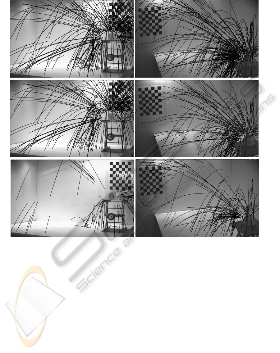
Figure 5: 3D matching. Left column: lateral camera. Right column: front-facing camera. Top row: all paths. Middle row:
matched paths. Bottom row: discarded paths. The paths were drawn on top of the first video frame to give an idea of the
relative location and orientation of the cameras.
iment), we necessarily discarded more paths from the
front view than from the lateral view. Of the paths
discarded from the lateral view (bottom row of Fig-
ure 5), most were travelling backwards or downwards
from the initial position of the target, i.e., toward re-
gions outside the view of the frontal camera. There-
fore, the apparent poor matching in this particular ex-
periment from Table 1 can be accounted for by paths
partially hidden from one of the cameras. It is also
worth noting that some of the discarded paths match
very closely to their own shadows (this can be seen in
the short path near the centre of the lower left image).
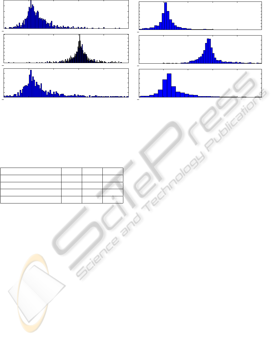
Figure 6 shows the reconstruction errors for all
points and paths obtained in the 48 experiments. The
left histogram plots the error (in cm) on the horizon-
tal axis against the number of points on the vertical
axis. The right-hand histogram shows the same pa-
rameters again, but with maximimum errors for each
path versus the number of paths. For most of the re-
constructed points, the reconstruction error is lower
than 5mm. Figure 7 shows the 3D reconstructions for
Experiments 1 and 2.
5.4 Validation by Inferring Parameters
If we assume constant acceleration, the position of a
droplet at time τ is given by
p(τ) =
p
x
(τ)
p
y
(τ)
p
z
(τ)
= p(0) + v(0)τ +
a
2
τ
2
. (11)
This model is not completely accurate as it ignores
viscous effects. However, (11) can still be used to
compute a rough estimate of the gravitational constant
ICPRAM 2012 - International Conference on Pattern Recognition Applications and Methods
150
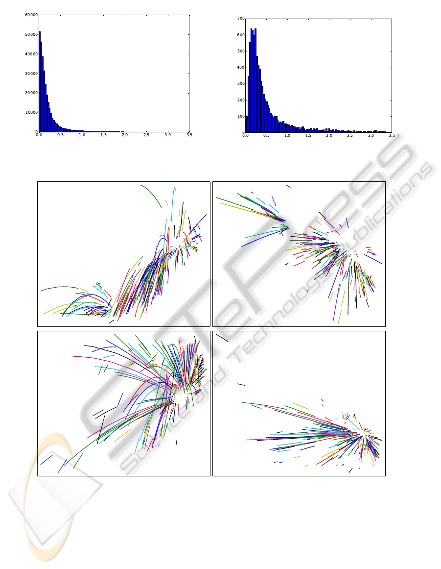
Figure 6: Error histograms. Left: Error in cm (horizontal axis) vs. the number of points (vertical axis). Right: Number of
paths (vertical axis) vs. maximum error in these paths.
Figure 7: 3D reconstruction of experiments 1 (top) and 2 (bottom). Left: lateral view. Right: top view.
g ≈ 9.8 m/s
2
. Notice we that we cannot use g directly
in our model-based prediction of image paths because
the parabolic paths constructed using Algorithm 1 be-
cause the paths constructed there are in image coordi-
nates.
From the frame-rate and our tracking data, we
know the locations p(τ) and times τ. Similarly as in
Section 3.3, we can fit each component of the data
points p(τ) with a parabola:
p(τ) ≈ d + e τ + f τ
2
. (12)
From (11) and (12), we can estimate the accelera-
tions as a ≈ 2f. When a droplet is ascending, both the
force of gravity and the drag force point downward.
Conversely, when a droplet is descending, the force
of gravity opposes the drag force. Thus, if we com-
pute the accelerations independently for upward and
downward portions of the trajectories, we should ob-
tain a greater magnitude for the vertical components
of acceleration in the first case than in the second.
Table 2 summarizes the mean vertical accelera-
EXTRACTION OF BLOOD DROPLET FLIGHT TRAJECTORIES FROM VIDEOS FOR FORENSIC ANALYSIS
151
5
0
5
10
15
20
0
10
20
30
40
50
5
0
5
10
15
20
0
5
10
15
20
25
30
35
40
5
0
5
10
15
20
0
10
20
30
40
50
60
x
y
z
5
0
5
10
15
20
0
50
100
150
200
250
300
350
400
450
5
0
5
10
15
20
0
50
100
150
200
250
300
5
0
5
10
15
20
0
100
200
300
400
500
600
x
y
z
Figure 8: Accelerations (in m/s
2
) computed from the 3D reconstruction. Left: using only the upwards portions of the paths.
Right: using only the downwards portions of the paths.
Table 2: Estimated value of g inferred from the paths, using
only the upwards portions, the downwards portions, and all
the points in the path, respectively. A constant acceleration
was assumed. Only sections of paths with at least 30 mea-
surements are used to compute these values. The number of
paths that had more than 30 measurements in each direction
are indicated in parentheses.
N. (up / down / all) Up Down Total
1 (19 / 111 / 120) 9.09 9.03 9.08
2 (69 /62 / 124) 10.41 9.13 9.85
3 (37 / 31 / 69) 9.93 7.84 9.04
T (1214 / 2486 / 3545) 10.36 10.24 10.36
tions obtained from the three experiments. Note that
the value is consistently greater in the upwards por-
tions than in the downwards portions, as expected.
Figure 8 is a histogram of the acceleration com-
ponents associated with each path extracted by the
experiments. Despite having obtained a good approx-
imation of g in the second row, the variance of the
computed values for the three axis shows that the ef-
fect of drag forces is not negligible and should be
taken into account when analyzing bloodstain pat-
terns in crime scenes.
6 CONCLUSIONS
We apply computer vision techniques to estimate pa-
rameters needed to describe blood droplet flight paths
caused by a violent event accurately. This paper rep-
resents the first step toward that goal: estimating 3D
trajectories of blood droplets using a stereo camera
setup. The system described here uses model-based
tracking to estimate trajectories of image features cap-
tured by individual cameras. The 2D image trajecto-
ries are then matched across the two cameras to re-
construct 3D trajectories in world coordinates. In a
given experiment, any proposed system needs to track
hundreds of droplets simultaneously; therefore, man-
ual annotation of ground truth to determine the per-
formance of the proposed algorithm is infeasible. In-
stead, we have developed three novel strategies for
indirectly measuring the performance of our system.
The initial results appear promising.
Several extensions of this work are currently in
progress. From our results, it is obvious that air resis-
tance and gravity play a significant role in how blood
droplets move through the air even at short distances.
We are currently developing physics-based models in-
corporating the influence of gravity and aerodynamic
drag to describe blood droplet trajectories. The data
acquired by the system described here can validate
putative physic-based motion models under devel-
opment and determine the relative magitude of the
forces ignored in stringing-based methods. Beyond
modelling droplet flight, it is necessary to investigate
robust methods based on a validated model for back-
tracking from a bloodstain to the original source.
REFERENCES
Balch, T., Khan, Z., and Veloso, M. (2001). Automati-
cally tracking and analyzing the behavior of live insect
colonies. In AGENTS ’01, pages 521–528. ACM.
Betke, M., Hirsh, D. E., Bagchi, A., Hristov, N. I., Makris,
N. C., and Kunz, T. H. (2007). Tracking large variable
numbers of objects in clutter. In CVPR ’07, pages 1–8.
IEEE.
Bevel, T. and Gardner, R. M. (2008). Bloodstain Pattern
Analysis With an Introduction to Crimescene Recon-
struction. CRC Press, 3
rd
edition.
ICPRAM 2012 - International Conference on Pattern Recognition Applications and Methods
152

Bijsterbosch, J. and Volgenant, A. (2010). Solving the rect-
angular assignment problem and applications. Ann.
Oper. Res., 181:443–462.
Bourgeois, F. and Lassalle, J.-C. (1971). An extension of
the Munkres algorithm for the assignment problem to
rectangular matrices. Commun. ACM, 14:802–804.
Bradski, G. (2000). The OpenCV Library. Dr. Dobbs J.
Buck, U., Kneubuehl, B., N
¨
ather, S., Albertini, N., Schmidt,
L., and Thali, M. (2011). 3D bloodstain pattern analy-
sis: Ballistic reconstruction of the trajectories of blood
drops and determination of the centres of origin of the
bloodstains. Forensic Sci. Int., 206(1-3):22–28.
Dasgupta, D., Hernandez, G., Garrett, D., Vejandla, P. K.,
Kaushal, A., Yerneni, R., and Simien, J. (2008). A
comparison of multiobjective evolutionary algorithms
with informed initialization and Kuhn-Munkres algo-
rithm for the sailor assignment problem. In GECCO
’08, pages 2129–2134. ACM.
Grover, D., Tower, J., and Tavar
´
e, S. (2008). O fly, where
art thou? J. Roy. Soc. Interface, 5(27):1181–1191.
Hartley, R. and Zisserman, A. (2004). Multiple view geom-
etry in computer vision. Cambridge University Press,
2
nd
edition.
Iwase, S. and Saito, H. (2004). Parallel tracking of all soccer
players by integrating detected positions in multiple
view images. In ICPR 2004, volume 4, pages 751–
754. IEEE.
Khan, Z., Balch, T., and Dellaert, F. (2003). Efficient parti-
cle filter-based tracking of multiple interacting targets
using an MRF-based motion model. In IROS 2003,
volume 1, pages 254–259. IEEE.
Khan, Z., Balch, T., and Dellaert, F. (2005a). MCMC-Based
Particle Filtering for Tracking a Variable Number of
Interacting Targets. IEEE Trans. Pattern Anal. Mach.
Intell., 27(11):1805–1918.
Khan, Z., Balch, T., and Dellaert, F. (2005b). Multitar-
get tracking with split and merged measurements. In
CVPR ’05, volume 1, pages 605–610. IEEE.
Kuhn, H. (1955). The Hungarian Method for the assignment
problem. Nav. Res. Logist., 2(1-2):83–97.
Munkres, J. (1957). Algorithms for the Assignment and
Transportation Problems. SIAM J. Appl. Math.,
5(1):32–38.
Nillius, P., Sullivan, J., and Carlsson, S. (2006). Multi-
Target Tracking–Linking Identities using Bayesian
Network Inference. In CVPR ’06, volume 2, pages
2187–2194.
Poore, A. B. and Gadaleta, S. (2006). Some assignment
problems arising from multiple target tracking. Math.
Comput. Model., 43(9-10):1074–1091.
Reid, D. (1979). An algorithm for tracking multiple targets.
IEEE Trans. Autom. Control, 24(6):843–854.
Straw, A. D., Branson, K., Neumann, T. R., and Dick-
inson, M. H. (2011). Multi-camera real-time three-
dimensional tracking of multiple flying animals. J.
Roy. Soc. Interface, 8(56):395–409.
Veenman, C., Reinders, M., and Backer, E. (2001). Resolv-
ing motion correspondence for densely moving points.
IEEE Trans. Pattern Anal. Mach. Intell., 23(1):54–72.
Yilmaz, A., Javed, O., and Shah, M. (2006). Object track-
ing: A survey. ACM Comput. Surv., 38(4).
EXTRACTION OF BLOOD DROPLET FLIGHT TRAJECTORIES FROM VIDEOS FOR FORENSIC ANALYSIS
153
