
CONVEX COMBINATIONS OF MAXIMUM MARGIN BAYESIAN
NETWORK CLASSIFIERS
Sebastian Tschiatschek and Franz Pernkopf
Department of Electrical Engineering, Laboratory of Signal Processing and Speech Communication
Graz University of Technology, Graz, Austria
Keywords:
Bayesian network classifiers, Discriminative learning, Convex relaxation, Maximum margin Bayesian
networks, Classifier enhancement, Combining weak classifiers.
Abstract:
Maximum margin Bayesian networks (MMBN) can be trained by solving a convex optimization problem
using, for example, interior point (IP) methods (Guo et al., 2005). However, for large datasets this training
is computationally expensive (in terms of runtime and memory requirements). Therefore, we propose a less
resource intensive batch method to approximately learn a MMBN classifier: we train a set of (weak) MMBN
classifiers on subsets of the training data, and then exploit the convexity of the original optimization problem
to obtain an approximate solution, i.e., we determine a convex combination of the weak classifiers.
In experiments on different datasets we obtain similar results as for optimal MMBN determined on all training
samples. However, in terms of computational efficiency (runtime) we are faster and the memory requirements
are much lower. Further, the proposed method facilitates parallel implementation.
1 INTRODUCTION
Endowing machine learning algorithms with the abil-
ity to generalize from prior observations is a difficult
problem in general. However, in the case of discrim-
inative classifiers, the support vector machine (SVM)
is a well established tool with good generalization
properties. The ability to generalize is achieved by
separating samples from distinct classes by a hyper-
plane that maximizes the margin between them.
While the large margin concept in SVMs was first
suggested by Vladimir Vapnik (Vapnik, 1998) in the
1960s, this idea of margin maximization has only re-
cently been introduced to Bayesian networks by Guo
et al. (Guo et al., 2005). In their paper they pro-
vided the basic definition of the margin in a proba-
bilistic environment as well as the formulation of a
convex optimization problem for learning maximum
margin Bayesian networks (MMBN). In contrast to
SVMs, for which lots of (efficient) training algo-
rithms have been proposed, e.g., (Platt, 1999; Shalev-
Shwartz et al., 2007) and many others, there is only
little literature on training MMBNs. Only two ap-
proaches are known in the community: the convex
optimization approach proposed by Guo et al. (Guo
et al., 2005) and a conjugate gradient based approach
by Pernkopf et al. (Pernkopf et al., 2011). While
the former approach provides slightly better classifi-
cation rates, it is computationally costly in terms of
runtime and memory consumption on large datasets
when directly solved by, e.g., interior point meth-
ods (Boyd and Lieven, 2004). Despite the lack of lit-
erature, MMBNs are serious competitors to SVMs as
they allow for the incorporation of domain knowledge
as well as efficient handling of missing features and
show comparable classification performance in vari-
ous experiments (Pernkopf et al., 2011).
In this paper we aim to present an algorithm that
approximately solves the convex formulation of the
MMBN learning problem, leading to good classifica-
tion results while being computationally less expen-
sive than the original formulation. This is achieved
by splitting the training set into subsets and subse-
quently training an MMBN on each of the subsets.
These MMBNs typically exhibit lower classification
performance than an MMBN trained on the whole
training set. However, the MMBNs can be combined,
by exploiting properties of the underlying optimiza-
tion problem, to form a stronger classifier. In ex-
periments we compare the performance of this ap-
proach with the performance of MMBNs trained on
the whole training set either by the convex formula-
tion or by the conjugate gradient based approach. In
most cases the classification rates of all three meth-
ods are competitive. Further experiments demonstrate
that the combined classifiers are naturally less prone
69
Tschiatschek S. and Pernkopf F. (2012).
CONVEX COMBINATIONS OF MAXIMUM MARGIN BAYESIAN NETWORK CLASSIFIERS.
In Proceedings of the 1st International Conference on Pattern Recognition Applications and Methods, pages 69-77
DOI: 10.5220/0003770300690077
Copyright
c
SciTePress

to overfitting and that they achieve good performance
on different partitions of the training set.
Many general schemes for combining classifiers
like Adaboost (Freund and Schapire, 1995), Bag-
ging (Breiman, 1996), Bayesian Model Averag-
ing (Bishop, 2007) exist. However, the basic prin-
ciple is quite different to our approach. While, for
example, Adaboost is based on the consecutive train-
ing of classifiers, each newly build classifier favoring
the missclassified samples of previous classifiers, our
approach is simply based on the properties of convex
optimization problems.
This paper is organized as follows: In Sect. 2 we
introduce the notation and briefly review the basic
concepts of Bayesian network classifiers. Based on
this, we introduce maximum margin Bayesian net-
work learning in Sect. 3. Subsequently, in Sect. 4
we propose a batch algorithm to reduce the computa-
tional and memory complexity of the training process.
Section 5 provides empirical results of the proposed
algorithm. Finally, Sect. 6 concludes the paper.
2 BAYESIAN NETWORK
CLASSIFIERS
A Bayesian network structure (BNS) (Koller and
Friedman, 2009) is a directed acyclic graph (DAG)
G = (V, E) consisting of nodes V and edges E. The
nodes represent random variables (RVs) Z
0
, . . . , Z
K
and the edges encode the dependenciesbetween them.
A joint probability distribution p over the same RVs
factorizes according to G , annotated as p ∼ G , if it
satisfies
p(Z
0
, . . . , Z
K
) =
K
∏
i=0
p(Z
i
|Π
G
(Z
i
)), (1)
where Π
G
(Z
i
) denotes the set of parents of Z
i
in
G (Koller and Friedman, 2009). All RVs are assumed
to take only discrete values from a finite set.
The tuple B = (G , p) is called a Bayesian network
(BN) if p ∼ G and p is specified by conditional prob-
ability distributions (CPDs) associated with the nodes
of G (Koller and Friedman, 2009). If it is not clear
from the context, we will annotate the graph G as G
B
and the probability distribution p as p
B
, to uniquely
identify these two objects with the corresponding BN
B .
A Bayesian network employed for classification
is a Bayesian network classifier. In such networks,
without loss of generality, let Z
0
represent the class
variable C ∈ C = {1, . . . , |C |}, where |C | is the num-
ber of classes. The other variables Z
1
, . . . , Z
K
are the
attributes of the classifier. Each of these attributes
Z
i
can take values in {1, . . . , |Z
i
|}. The random vec-
tor Z consists of the attributes of the classifier, i.e.,
Z = [Z
1
, . . . , Z
K
]. An instantiation of Z is denoted
by z and is a specific assignment of values to the
random variables. Bold face letters refer to sets of
variables while regular letters denote single variables.
The CPDs associated with the nodes of G describing
the probability distribution p can be parameterized by
a vector θ with entries θ
j
i|h
denoting specific condi-
tional probabilities. That is,
θ
j
i|h
= p(Z
j
= i|Π
G
(Z
j
) = h),
where Π
G
(Z
j
) = h means that the parents of random
variable Z
j
take their h
th
assignment (lexicographi-
cally ordered). To make the connection between p
and θ explicit, we will typically append the subscript
θ to p, i.e., p
θ
. Given an unlabeled sample z the class
is predicted as the maximum aposteriori (MAP) esti-
mate, i.e., as
argmax
c∈C
p
θ
(C = c|Z = z) = argmax
c∈C
p
θ
(C = c, Z = z),
(2)
where the last equality follows because the normal-
ization term
∑
z
p
θ
(Z = z) is constant for all classes.
To employ BNs for classification two problems
must be solved:
1. Structure Learning: Identify BNSs that appro-
priately model the dependencies in the considered
data and facilitate discrimination. This resorts to
discrete optimization problems.
2. Parameter Learning: Given a BNS, determine
probability distributions that factorize according
to the structure and yield good classification re-
sults. Parameter learning gives rise to continuous
optimization problems.
These problems can be solved independently or
jointly. In this paper we do not solve the first prob-
lem, but assume a fixed BNS to be given. Anyway,
the interested reader can find additional information
on this, e.g., in (Acid et al., 2005).
Parameter Learning
There are two different approaches to parameter
learning in BNs, namely generative and discrimina-
tive ones. To briefly describe both approaches, let G
be a fixed BNS and T = {(c
(n)
, z
(n)
) : 1 ≤ n ≤ N} a
training set consisting of N i.i.d. labeled training sam-
ples, i.e., N instances of values of the RVs represented
by the nodes of G .
ICPRAM 2012 - International Conference on Pattern Recognition Applications and Methods
70

Generative Parameter Learning. The goal of gen-
erative parameter learning is to identify probability
distributions p ∼ G that model the joint probability
of the classifier attributes and the corresponding class
label appropriately. A standard method to find such a
distribution, is maximum likelihood parameter learn-
ing (Pearl, 1988), where p is determined as
p
B
= argmax
p
′
∼G
N
∏
n=1
p
′
(c
(n)
, z
(n)
). (3)
Discriminative Parameter Learning. Discrimina-
tive approaches aim at learning the class poste-
rior probability p(c|z) directly. One representa-
tive of discriminative parameter learning approaches
is conditional likelihood (CL) parameter learning
that is tightly connected to minimizing empirical
risk (Greiner et al., 2005). In CL learning the proba-
bility distribution p is determined as
p
B
= argmax
p
′
∼G
N
∏
n=1
p
′
(c
(n)
|z
(n)
), (4)
i.e., the conditional likelihood of the classes given the
attributes is maximized over the samples in the train-
ing set.
Another objective for discriminative parameter
learning is the maximum margin criterion. It is de-
scribed in detail in the next section. Generally, dis-
criminative scores such as the margin or CL are not
decomposable as the likelihood for maximum likeli-
hood learning. Consequently, there is no closed form
solution for discriminative parameter learning and it-
erative optimization tools are required.
3 MAXIMUM MARGIN
BAYESIAN NETWORKS
The idea behind maximum margin parameter learn-
ing is to identify a probability distribution p such that
the minimal separation between samples from differ-
ent classes is maximized. This approach is inspired
by SVMs, for which one tries to maximize the mar-
gin between samples from different classes. In the
case of SVMs the margin is typically the distance be-
tween the feature space representation of the consid-
ered samples in some appropriate norm. For Bayesian
networks, following the approach taken in (Guo et al.,
2005), the margin can be defined as a ratio of proba-
bilities (also named conditional likelihood ratio):
Definition 1. The multi-class margin of the labeled
sample (c, z) in the Bayesian Network B is
d
B
(c, z) = min
c
′
∈C ,c
′
6=c
p
B
(c|z)
p
B
(c
′
|z)
= min
c
′
∈C ,c
′
6=c
p
B
(c, z)
p
B
(c
′
, z)
.
(5)
Informally, the margin measures how much more
likely the sample belongs to the correct class c than to
the most likely competing class.
Using this definition, a MMBN can be defined as
a BN that maximizes the minimum margin between
any two samples from different classes of the training
set.
Definition 2. Let T be a given training set with N
training samples and G a given BNS. Then, B =
(G , p) is a maximum margin Bayesian network if B
is a BN and p is an optimal solution of the problem
maximize
p
′
∼G
N
min
n=1
d
B
(c
(n)
, z
(n)
). (6)
There exists only little literature dealing with
the problem of learning MMBNs. Pernkopf et
al. (Pernkopf et al., 2011) solved it using a conju-
gate gradient based method while Guo et al. (Guo
et al., 2005) reformulated the margin optimization as
a convex optimization problem. The former method
is superior in terms of computation speed and mem-
ory requirements, but the convex formulation re-
sults in slightly better classifiers (Pernkopf et al.,
2011). Therefore, it is desireable to solve the con-
vex optimization problem, at least approximately, in a
resource-saving way. We present an approach to this
in Sect. 4.
Convex Formulation of Maximum Margin
Bayesian Networks
The maximum margin learning problem is formulated
as a convex optimization problem by introducing a
parameter vector w with elements w
j
i|h
= log(θ
j
i|h
) (in
some arbitrary, but fixed order). Using the same order
of the elements, the feature vectors φ(c
(n)
, z
(n)
) with
elements
u
j,n
i|h
= 1
{z
(n)
j
=i and Π
G
(Z j)
(n)
=h}
,
can be defined. The symbol 1
{cond}
denotes the in-
dicator function, i.e., it equals 1 if and only if cond
is true and 0 otherwise. Then, the probability of any
sample (c
(n)
, z
(n)
) of the BN can be written as
p
θ
(c
(n)
, z
(n)
) = exp(φ(c
(n)
, z
(n)
)
T
w),
where (·)
T
denotes the transposition operator. Using
this, the logarithm of the multi-class margin of the n
th
CONVEX COMBINATIONS OF MAXIMUM MARGIN BAYESIAN NETWORK CLASSIFIERS
71

sample from the training set in (5) becomes
logd
B
(c
(n)
, z
(n)
) =
min
c∈C ,c6=c
(n)
h
φ(c
(n)
, z
(n)
) − φ(c, z
(n)
)
i
T
w. (7)
Hence, the criterion given in (6) can be reformulated
as
maximize
γ,w
γ (8)
s.t. ∆
n,c
w ≥ γ, ∀n and c 6= c
(n)
(9)
|Z
j
|
∑
i=1
exp(w
j
i|h
) = 1, ∀ j, h (10)
γ ≥ 0, (11)
where γ is the logarithm of the minimum of all sample
margins and
∆
n,c
=
h
φ(c
(n)
, z
(n)
) − φ(c, z
(n)
)
i
T
.
The constraints (9) ensure that all sample margins are
larger than γ. Together with the constraint γ ≥ 0 it is
explicitly required that all sample margins are larger
than one (zero in logarithmic scale), i.e., all samples
are classified correctly. This can only be achieved
for separable data. For non-separable data the above
problem is infeasible. The constraints (10) ensure that
w describes a valid probability distribution, i.e., all
conditional probabilities in the BN sum to 1. Note
that the dependency of w on θ was dropped. In this
way, solving the above problem leads to a vector w
that describes a probability distribution p such that
p ∼ G and B = (G , p) is an MMBN network.
The above problem is still not convex because of
the constraints (10). However, these constraints can
be relaxed by replacing the equality by an inequality
resulting in a convexproblem. Further, one slack vari-
able ε
n
for each training sample (c
(n)
, z
(n)
) to account
for non-separable data is introduced. Rewriting the
objective, we obtain the optimization problem (more
details are given in the paper (Guo et al., 2005))
minimize
γ,ε
1
,...,ε
N
,w
1
2γ
2
+ B
N
∑
n=1
ε
n
(12)
s.t. ∆
n,c
w ≥ γ − ε
n
, ∀n and c 6= c
(n)
(13)
|Z
j
|
∑
i=1
exp(w
j
i|h
) ≤ 1, ∀ j, h (14)
ε
n
≥ 0, ∀n, (15)
γ ≥ 0, (16)
where B ≥ 0 is a parameter to control the slack-effect,
i.e., a tradeoff parameter between a large margin and
large sample slacks (similar to the parameter C in
SVMs). We also refer to B as the regularization pa-
rameter.
Because of the relaxed constraints
|Z
j
|
∑
i=1
exp(w
j
i|h
) ≤ 1, ∀ j, h,
in (12) the vector w of an optimal solution does not
necessarily describe valid CPDs. That is, w can rep-
resent a subnormalized probability distribution (abus-
ing terminology). However, for some network struc-
tures, e.g., Naive Bayes and Tree Augmented Net-
works, the resulting parameter vector w allows for
renormalization without changing the decision func-
tion in (2). For more details we refer the interested
reader to (Roos et al., 2005).
4 CONVEX COMBINATION OF
WEAK MMBNS
4.1 Discussion of Sample/Feature Size
Equation (12) represents a convex optimization prob-
lem that can be solved by any minimization method
allowing for a nonlinear objective and nonlinear con-
vex inequality constraints. For example, interior point
methods (Boyd and Lieven, 2004) are such a class of
methods. While these methods are efficient in theory,
Pernkopf et al. (Pernkopf et al., 2011) observed large
computational requirements when learning MMBNs
parameters using the convex formulation. This is es-
pecially true for large training sets in terms of samples
and/or features:
• The total number of unknowns in the optimization
problem is 1+N+Var(G ), where Var(G ) denotes
the number of variables required to fully specify
the conditional probability tables associated with
the nodes of G in a BN. Hence, Var(G ) is large
for dense network structures and structures with
many RVs and/or large cardinalities of the RVs.
Large values of 1 + N + Var(G ) lead to high di-
mensional search spaces, typically resulting in
long runtimes for the optimization process.
• Despite the non-negativity constraints on γ and
ε
1
, . . . , ε
N
, there is one nonlinear inequality con-
straint for each conditional probability of the net-
work. Additional, for every training sample |C |
linear inequality constraints are required.
The number of inequalities of the convex formu-
lation influences the required number of iterations
ICPRAM 2012 - International Conference on Pattern Recognition Applications and Methods
72

for interior point methods to converge to a so-
lution with specific accuracy (Boyd and Lieven,
2004). Larger numbers of inequality constraints
lead to larger number of iterations.
4.2 Proposed Batch Strategy
To reduce the computational burden we propose to ap-
ply a batch algorithm. The idea behind the algorithm
is to train a sequence of weak classifiers, each on a
subset of the training set using the convex formulation
in (12). Subsequently, these classifiers are combined
to form a strong classifier.
Given a BNS G , the number M ∈ N of weak clas-
sifiers to train and a regularization parameter B ≥ 0,
the algorithm performs the following steps:
1. Determine a cover T = {T
1
, . . . , T
M
} of T , i.e., T
is comprised of M subsets of the training set such
that
T =
M
[
m=1
T
m
.
2. Train M classifiers on the partial training sets, i.e.,
determine γ
m
, ε
m
, w
m
as solutions to (12) using
training set T
m
.
3. Determine an optimal convex combination of the
M classifiers such that the original objective is
minimized. Therefore, determine α
1
, . . . , α
M
as
the optimization variables that solve
minimize
α
′
1
,...,α
′
M
MMBN
M
∑
m=1
α
′
m
w
m
!
+ R, (17)
s.t. α
′
1
, . . . , α
′
M
≥ 0, (18)
α
′
1
+ . . . + α
′
M
= 1, (19)
where
R := D
s
M
∑
m=1
α
m
−
1
M
2
(20)
and MMBN(w) is the minimization problem (12)
with fixed w, i.e.,
minimize
γ,ε
1
,...,ε
N
1
2γ
2
+ B
N
∑
n=1
ε
n
(21)
s.t. ∆
n,c
w ≥ γ − ε
n
, ∀n and c 6= c
(n)
γ ≥ 0,
|Z
j
|
∑
i=1
exp(w
j
i|h
) ≤ 1, ∀ j, h,
ε
n
≥ 0, ∀n.
The parameter D ≥ 0 can be used to ensure that
all weak classifiers participate in the final clas-
sifier. Selecting large values for D results in
all weak classifiers being equally weighted when
constructing the final classifier. Hence, the sec-
ond term in (17) can be viewed as a regularization
term.
The constraints on the coefficients α
′
1
, . . . , α
′
M
,
i.e., nonnegativity (18) and sum to one (19), are
required for convex combinations of w
1
, . . . , w
M
.
In this way the convex hull defined as the set of all
convex combinations of w
1
, . . . , w
M
is searched
for an optimal parameter vector w
′
in the sense
of (21). Considering not arbitrary linear combina-
tions of w
i
but only convex combinations ensures
that the vector w
′
=
∑
M
m=1
α
′
i
w
i
satisfies the sub-
normalization constraints of the original convex
formulation.
Equation (21) essentially describes a one-
dimensional optimization problem and can be
solved easily. Details can be found in the Ap-
pendix.
4. Return the BN specified by B = (G , p(w)), where
w =
M
∑
m=1
α
m
w
m
. (22)
and p(w) is the probability distribution obtained
from w by renormalization.
4.3 Geometric Interpretation of the
Batch Algorithm
Figure 1 illustrates the principle of the proposed batch
algorithm in a two dimensional parameter space for
D = 0. The parameters of an optimal classifier in
the sense of (12) are indicated by a plus sign and the
parameters of the weak classifiers found by splitting
the overall training set into four subsets are shown as
grey circles. The objective to be minimized is visu-
alized by contour lines, where the optimal classifier
is able to detect the global optimum. Solving (17)
corresponds to searching the gray shaded region, i.e.,
searching the convex hull spanned by the parameters
of the weak classifiers. In the shown example, the pa-
rameters marked by the diamond are the optimal ones
in the convex hull, i.e., the parameters with the mini-
mal objective.
If the parameters of the optimal classifier would
lie in the convex hull, then the proposed algorithm
would find the optimal solution. While it seems rea-
sonable that this occurs in low dimensional parameter
spaces, this will typically not happen in high dimen-
sional spaces; in the case of the USPS database we
have a ∼ 3000 dimensional parameter space. Having
trained, for example, 40 weak classifiers only a small
CONVEX COMBINATIONS OF MAXIMUM MARGIN BAYESIAN NETWORK CLASSIFIERS
73

subset of the parameter space lies in the spanned con-
vex hull making it very unlikely that a global mini-
mum is found. Clearly, the performance of the pro-
posed batch algorithm depends on the selected cover
and on the determined weak classifiers. Training of
the weak classifiers such that the spanned region cov-
ers good classifiers is subject to future work.
Figure 1: Geometric interpretation of the proposed batch
algorithm.
5 EXPERIMENTS
We present classification results for frame-based pho-
netic data using the TIMIT speech corpus and for
handwritten digit recognition using the USPS and
MNIST datasets. The experiments were performed
using a fixed Bayesian network structure, namely a
naive Bayes (NB) classifier structure. The NB struc-
ture is illustrated in Fig. 2. All attributes Z
1
, . . . , Z
K
are conditionally independent given the class. While
the structure is simple, good performance can be
achieved in various applications even if the condi-
tional independence assumptions are unrealistic or
even false in most of the data (Rish, 2001).
C
Z
1
Z
2
Z
3
· · · Z
K
Figure 2: Naive Bayes network.
5.1 Simulation Setup
We used IPOPT (Interior Point OPtimizer) (W¨achter
and Biegler, 2005), a freely available software pack-
age for large-scale optimization that showed good
performance in various applications to solve the op-
timization problem (12). IPOPT requires a linear
solver to compute the step-directions in the applied
interior point method. In our experiments, we em-
ployed PARDISO (Schenk and G¨artner, 2004; Schenk
and G¨artner, 2006; Karypis and Kumar, 2006) for this
purpose. The optimization problem (17) was solved
using the function
fmincon
included in the optimiza-
tion toolbox from Matlab. Furthermore, the cover
of the training set in the batch algorithm was deter-
mined as follows: The training set was split into M
equally sized disjoint subsets. The samples in each
subset were selected according to the prior class prob-
abilities. CPU time experiments were performed on
a personal computer with 2.8 GHz, 32 GB of mem-
ory and exploiting (multicore) parallelization of up to
11 cores. The parallelization especially results in a
speedup of the linear solver PARDISO. The reported
CPU times are those reported by IPOPT and Mat-
lab. The regularization parameter B was selected us-
ing cross tuning for the TIMIT data, while fixed as
B = 1 for the USPS and MNIST data.
5.2 Datasets
In our experiments we considered the MNIST, USPS
and TIMIT databases, that we briefly describe in the
following:
• TIMIT-4/6 Data. This dataset is extracted from
the TIMIT speech corpus using the dialect speak-
ing region 4 which consists of 320 utterances
from 16 male and 16 female speakers. Speech
frames are classified into either four or six pho-
netic classes using 110134 and 121629 samples,
respectively. Each sample is represented by 20
mel-frequency cepstral coefficients (MFCCs) and
wavelet-based features. We perform classification
experiments on data of male speakers (Ma), fe-
male speakers (Fe), and both genders (Ma+Fe),
all in all resulting in 6 distinct data sets (i.e., Ma,
Fe, Ma+Fe, each with 4 and 6 classes). The data
have been split into two mutually exclusive sub-
sets where 70 % of the data is used for training
and 30 % for testing. More details about the fea-
tures can be found in (Pernkopf et al., 2009).
• USPS Data. This dataset contains 11000 uni-
formly distributed handwritten digit images from
zip codes of mail envelopes. The database is split
into 8000 images for training and 3000 for testing.
Each digit is represented as a 16 × 16 grayscale
image, where each pixel is considered as feature.
• MNIST Data (LeCun et al., 1998). This dataset
contains 60000 samples for training and 10000
samples for testing of handwritten digits. To re-
duce computation time we reduced the training
set to 10000 samples according to the prior class
ICPRAM 2012 - International Conference on Pattern Recognition Applications and Methods
74

60
65
70
75
80
85
90
95
100
W1
W2
W3
W4
W5
W6
W7
W8
W9
W10
W11
W12
W13
W14
W15
W16
W17
W18
W19
W20
F
classification rate
Figure 3: Classification performance in [%] of the proposed batch algorithm on the USPS dataset. The classification rates on
the complete training set (light grey bars) and on the test set (dark grey bars) of the weak classifiers (labeled as ”W1“, . . .,
”W20“) and of the final classifier (labeled as F) are shown. The light gray horizontal line marks the average classification
rate of the weak classifiers on the training set and the dark gray horizontal line the average classification rate on the test set,
respectively.
Table 1: Classification rates CR in [%] for different datasets and number of splits M. The columns CT shows the total CPU
time for the parameter learning, the column CT
max
the maximum CPU time for learning a single weak classifier and CT
conv
the CPU time for finding the optimal convex combination of the weak classifiers (all times are given in seconds).
Database M CT CR M B D CT
max
CT
conv
CT CR
MNIST 1 20152 86.01 100 1 1· 10
5
52 2180 5380 83.99
USPS 1 89364 90.90 20 1 1· 10
3
1494 388 25599 88.10
TIMIT Ma+Fe-4 1 3811 92.23 40 4· 10
−3
1· 10
3
105 1115 4315 92.05
TIMIT Ma-4 1 2576 93.06 20 4· 10
−3
1· 10
3
51 230 1072 92.95
TIMIT Fe-4 1 1502 91.82 20 4· 10
−3
1· 10
3
55 310 1296 91.64
TIMIT Ma+Fe-6 1 19574 85.61 40 4· 10
−3
1· 10
6
612 1432 21952 85.45
TIMIT Ma-6 1 10285 86.67 20 4· 10
−3
1· 10
6
207 240 3886 86.11
TIMIT Fe-6 1 9676 85.36 20 4· 10
−3
7· 10
5
214 503 3912 85.13
probabilities. The digits respresented by gray-
level images were down-sampled by a factor of
two resulting in a resolution of 14× 14 pixels, i.e.,
196 features.
5.3 Classification Results on the USPS
Data
We appliedthe proposed batch algorithm on the USPS
dataset by training 20 weak classifiers. The regu-
larization parameter was selected as B = 1 (without
applying any parameter-tuning method). The perfor-
mance in terms of the classification rate of the weak
classifiers on the complete training and the test set is
shown in Fig. 3. Additionally, the performance of the
final classifier determined by solving (17) is shown.
The final classifier has a 15 to 25 percent better
classification rate than the weak classifiers (on the
training, as well as, on the test set).
1
All of the weak
1
However, note that the performance gain of the final
classifiers achieved a classification rate of 100 per-
cent on the training set T
m
they were trained on (not
shown in the figure) indicating overfitting. In contrast
to this, the final classifier avoids this problem. This
is also observed in other algorithms that combine the
results of several classifiers like bagging and boost-
ing (Breiman, 1996; Freund and Schapire, 1995).
5.4 Classification Results for Various
Databases
Classification results for the TIMIT, USPS and
MNIST database are presented in Tab. 1. Further,
the required CPU times for the parameter learning
are shown. Note that running the proposed batch al-
gorithm with M = 1 is equal to solving the original
convex optimization problem (12). Hence, classifiers
trained by the proposed algorithm perform slightly
classifier is not always as impressive as in this case, e.g., on
the order of 3 to 10 percent on the TIMIT datasets.
CONVEX COMBINATIONS OF MAXIMUM MARGIN BAYESIAN NETWORK CLASSIFIERS
75
worse than classifiers trained on the whole training
sets. Nevertheless, the classification rates are com-
petitive.
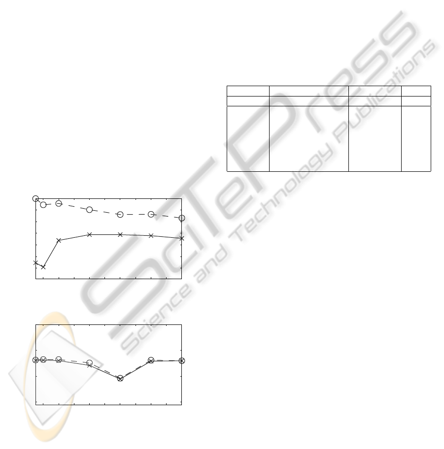
5.5 Classification Results for Different
Partitionings
For this experiment the USPS and TIMIT Ma-4 data
was considered. The number of training samples of
the whole training set was reduced to 1000 samples
in the case of the USPS data. The parameters B and
D were selected as in Tab. 1. Classification results for
the two datasets and for varying number of splits M of
the training set are shown in Fig. 4. For USPS data the
classification rate on the training set decreases with
an increasing number of splits while the classification
rate on the test set increases. This indicates overfit-
ting for low values of M. For TIMIT data a region
(M = 12 in the plot) can be identified in which both
the classification rate on the training and on the test
set decreases. For this region, the convex hull of the
determined weak classifiers does not contain a strong
classifiers for the complete training set. Clearly, to
achieve optimal performance for all different parti-
tionings the parameters B and D would have to be
retuned for every partitioning.
2 4 6 8 10 12 14 16 18 20
70
75
80
85
90
95
100
Number of splits
Classification rate
(a) USPS data (only 1000 training samples used)
2 4 6 8 10 12 14 16 18 20
85
90
95
100
Number of splits
Classification rate
(b) TIMIT-4/6 Ma-4 database
Figure 4: Classification rate in [%] on the training set
(dashed line) and on the test set (solid line) for different
numbers of splits of the training set.
5.6 Comparison to Conjugate Gradient
MMBN and SVMs
Table 2 compares the classification results of the pro-
posed algorithm, the conjugate gradient MMBN al-
gorithm (CG-MMBN) (Pernkopf et al., 2011) and
SVMs (with fixed parameters C
∗
= 1, σ = 0.05)
on the TIMIT-4/6 data. SVMs slightly outperform
the MMBNs in all cases. The proposed algorithm
achieves approximately the same classification rates
as CG-MMBN.
Table 2: Classification rates CR in percent for different
TIMIT-4/6 datasets and different classifiers. The columns
M and D show the parameters supplied to the proposed
batch algorithm. The parameter B = 4· 10
−3
in all experi-
ments.
proposed MMBN CG-MMBN SVM
Database M D CR CR CR
Ma+Fe-4 40 1· 10
3
92.05 92.09 92.49
Ma-4 20 1·10
3
92.95 92.97 93.30
Fe-4 20 1· 10
3
91.64 91.57 92.14
Ma+Fe-6 40 1· 10
6
85.45 85.41 86.24
Ma-6 20 1·10
6
86.11 86.20 87.19
Fe-6 20 7· 10
5
85.13 84.85 86.19
6 CONCLUSIONS
We proposed a batch method for approximately learn-
ing maximum margin Bayesian networks using a con-
vex formulation. The method is less computation-
ally demanding than solving the original formula-
tion. Still, the obtained results are comparable, as
demonstrated in various experiments. Further, the
method facilitates parallel implementation as training
the weak classifiers could be fully parallelized.
Since the presented results are quite promising,
we plan to address the following problems:
• Derivation of generalization bounds for MMBNs
trained by the convex combination scheme.
• Does an optimal cover C of T exist, i.e., a cover
that will result in a best possible classifier?
• Performing further experiments, especially on
more general network structures.
ACKNOWLEDGEMENTS
This work was supported by the Austrian Science
Fund (project number P22488-N23).
ICPRAM 2012 - International Conference on Pattern Recognition Applications and Methods
76

REFERENCES
Acid, S., Campos, L. M., and Castellano, J. G. (2005).
Learning Bayesian network classifiers: Searching in
a space of partially directed acyclic graphs. Machine
Learning, 59:213–235.
Bishop, C. M. (2007). Pattern Recognition and Ma-
chine Learning (Information Science and Statistics).
Springer, 1st ed. 2006. corr. 2nd printing edition.
Boyd, S. and Lieven, V. (2004). Convex Optimization. Cam-
bridge University Press.
Breiman, L. (1996). Bagging predictors. Machine Learn-
ing, 24(2):123–140.
Freund, Y. and Schapire, R. E. (1995). A decision-theoretic
generalization of on-line learning and an application
to boosting.
Greiner, R., Su, X., Shen, B., and Zhou, W. (2005). Struc-
tural extension to logistic regression: Discriminative
parameter learning of belief net classifiers. Machine
Learning, 59(3):297–322.
Guo, Y., Wilkinson, D., and Schuurmans, D. (2005). Max-
imum margin Bayesian networks. In Proceedings of
the 21th Annual Conference on Uncertainty in Artifi-
cial Intelligence, pages 233–242. AUAI Press.
Karypis, G. and Kumar, V. (2006). A fast and high quality
multilevel scheme for partitioning irregular graphs,.
SIAM Journal on Scientific Computing, 20(1):359–
392.
Koller, D. and Friedman, N. (2009). Probabilistic Graphi-
cal Models: Principles and Techniques. MIT Press.
LeCun, Y., Bottou, L., Bengio, Y., and Haffner, P. (1998).
Gradient-based learning applied to document recogni-
tion. Proceedings of the IEEE, 86(11):2278–2324.
Pearl, J. (1988). Probabilistic Reasoning in Intelligent Sys-
tems: Networks of Plausible Inference. Morgan Kauf-
mann Publishers Inc., San Francisco, CA, USA.
Pernkopf, F., Van Pham, T., and Bilmes, J. A. (2009). Broad
phonetic classification using discriminative Bayesian
networks. Speech Communication, 51(2):151–166.
Pernkopf, F., Wohlmayr, M., and Tschiatschek, S. (2011).
Maximum margin bayesian network classifiers. IEEE
Transactions on Pattern Analysis and Machine Intel-
ligence, (accepted).
Platt, J. (1999). Sequential minimal optimization: A fast
algorithm for training support vector machines. Ad-
vances in Kernel Methods-Support Vector Learning,
pages 1–21.
Rish, I. (2001). An empirical study of the naive Bayes clas-
sifier. In IJCAI 2001 Workshop on Empirical Methods
in Artificial Intelligence, pages 41–46.
Roos, T., Wettig, H., Gr¨unwald, P., Myllym¨aki, P., and Tirri,
H. (2005). On Discriminative Bayesian Network Clas-
sifiers and Logistic Regression. Machine Learning,
59(3):267–296.
Schenk, O. and G¨artner, K. (2004). Solving unsymmet-
ric sparse systems of linear equations with PARDISO.
Future Generation Computer Systems, 20(3):475–
487.
Schenk, O. and G¨artner, K. (2006). On fast factoriza-
tion pivoting methods for symmetric indefinite sys-
tems. Electronic Transactions on Numerical Analysis,
23:158–179.
Shalev-Shwartz, S., Singer, Y., and Srebro, N. (2007). Pega-
sos: Primal estimated sub-gradient solver for svm. In
Proceedings of the 24th international conference on
Machine learning, pages 807–814. ACM.
Vapnik, V. N. (1998). Statistical Learning Theory. Wiley-
Interscience.
W¨achter, A. and Biegler, L. T. (2005). On the implemen-
tation of an interior-point filter line-search algorithm
for large-scale nonlinear programming. Mathematical
Programming, 106(1):25–57.
APPENDIX
Solving the Intermediate Optimization
Problem
The optimization problem (21) for fixed w satisfying
the subnormalization constraints and given training
set T of N samples can be rewritten as
minimize
γ,ε
1
,...,ε
N
1
2γ
2
+ B
N
∑
n=1
ε
n
(23)
s.t. ex
n,c
≥ γ − ε
n
, ∀n and c 6= c
(n)
γ ≥ 0, ε
n
≥ 0, ∀n,
where we set ex
n,c
= ∆
n,c
w. For n = 1, . . . , N let
x
n
= min
c∈C ,c6=c
(n)
ex
n,c
.
Then, the above problem is equivalent to
minimize
γ,ε
1
,...,ε
N
1
2γ
2
+ B
N
∑
n=1
ε
n
(24)
s.t. x
n
≥ γ − ε
n
, ∀n
γ ≥ 0, ε
n
≥ 0, ∀n,
because the removed constraints will be simultane-
ously satisfied. In an optimal solution with margin γ
′
the term
∑
N
n=1
ε
n
must be as small as possible. There-
fore, all the ε
n
are required to take the minimal value
that is still feasible. This is ε
n
= γ
′
− x
n
, if this quan-
tity is positive. Or ε
n
= 0 otherwise. In this way, the
optimization problem becomes
minimize
γ
1
2γ
2
+ B
N
∑
n=1
max{γ− x
n
, 0} (25)
s.t. γ ≥ 0
and can be easily solved. If required, the slacks ε
n
can
subsequently be calculated as ε
n
= max{γ− x
n
, 0}.
CONVEX COMBINATIONS OF MAXIMUM MARGIN BAYESIAN NETWORK CLASSIFIERS
77
