OBJECT RECOGNITION IN PROBABILISTIC 3-D VOLUMETRIC

SCENES

Maria I. Restrepo

∗

, Brandon A. Mayer

†

and Joseph L. Mundy

‡

School of Engineering, Brown University, 182 Hope Street, Providence, RI, U.S.A.

Keywords:

3-d Object recognition, 3-d Data processing, Machine vision, Bayesian learning.

Abstract:

A new representation of 3-d object appearance from video sequences has been developed over the past several

years (Pollard and Mundy, 2007; Pollard, 2008; Crispell, 2010), which combines the ideas of background

modeling and volumetric multi-view reconstruction. In this representation, Gaussian mixture models for in-

tensity or color are stored in volumetric units. This 3-d probabilistic volume model, PVM, is learned from a

video sequence by an on-line Bayesian updating algorithm. To date, the PVM representation has been applied

to video image registration (Crispell et al., 2008), change detection (Pollard and Mundy, 2007) and classiﬁca-

tion of changes as vehicles in 2-d only (Mundy and Ozcanli, 2009;

Ozcanli and Mundy, 2010). In this paper,

the PVM is used to develop novel viewpoint-independent features of object appearance directly in 3-d. The

resulting description is then used in a bag-of-features classiﬁcation algorithm to recognize buildings, houses,

parked cars, parked aircraft and parking lots in aerial scenes collected over Providence, Rhode Island, USA.

Two approaches to feature description are described and compared: 1) features derived from a PCA analysis

of model neighborhoods; and 2) features derived from the coefﬁcients of a 3-d Taylor series expansion within

each neighborhood. It is shown that both feature types explain the data with similar accuracy. Finally, the

effectiveness of both feature types for recognition is compared for the different categories. Encouraging ex-

perimental results demonstrate the descriptive power of the PVM representation for object recognition tasks,

promising successful extension to more complex recognition systems.

1 INTRODUCTION AND PRIOR

WORK

A semantic description of 3-d scenes is essential to

many urban and surveillance applications. This pa-

per presents a new volumetric representation for the

description of 3-d scenes that captures the probabilis-

tic nature of 3-d reconstruction from multiple image

views and video sequences. A recognition approach is

described to provide semantic labels for aerial scenes

including such categories as houses, buildings, parked

cars, and parked aircraft. The labels are found by an

object classiﬁcation algorithm based on features ex-

tracted directly from a 3-d representation of scene ap-

pearance. The resulting object-centered recognition

model combines the probability of surface appearance

and surface occupancy at densely sampled locations

in 3-d space, thus incorporating the ambiguity inher-

ent in surface reconstruction from imagery. To the

authors’ knowledge, this paper represents the ﬁrst

——————————-

∗

†

Ph.D. Student

‡

Professor of Engineering

attempt to base scene classiﬁcation on a volumetric

probabilistic model that learns, in a dense manner, the

appearance and geometric information of 3-d scenes

from images.

In related work, many 3-d object recognition algo-

rithms have been developed in recent years to search

the rapidly growing databases of 3-d models (Pa-

padakis et al., 2010; Shapira et al., 2010; Drost et al.,

2010; Bariya and Nishino, 2010; Bronstein et al.,

2011). These recognition algorithms operate on mod-

els that are synthetically generated or obtained in a

controlled environment using 3-d scanners. Through-

out most of the object-retrieval literature, the domi-

nant representation of 3-d geometry is a mesh or point

cloud, where the intrinsic properties of the represen-

tation are used to describe shape models. However,

neither of these representations is able to express the

uncertainty and ambiguity of 3-d surfaces inherent in

reconstruction from aerial image sequences.

Other recent works have favored volumetric shape

180

I. Restrepo M., A. Mayer B. and L. Mundy J. (2012).

OBJECT RECOGNITION IN PROBABILISTIC 3-D VOLUMETRIC SCENES.

In Proceedings of the 1st International Conference on Pattern Recognition Applications and Methods, pages 180-190

DOI: 10.5220/0003776301800190

 SciTePress

descriptors to better cope with isometric deformations

(Raviv et al., 2010), and to improve segmentation of

models into parts and matching of parts from differ-

ent objects (Shapira et al., 2010). However, the volu-

metric cues of Raviv and Shapira are deﬁned by an

enclosing boundary (represented by a mesh). The

probabilistic volume model, PVM, used in this work,

learns geometry and appearance in a general frame-

work that can handle changes in viewpoint, illumina-

tion and resolution, without regard to surface topol-

ogy. Therefore, this work addresses the problem of

categorizing static objects in scenes learned from im-

ages collected under unrestricted conditions, where

the only requirement is known camera calibration ma-

trices. It is worth pointing out that the volumetric rep-

resentation used in this work is different from a rep-

resentation obtained from a range scanner, not only

in that appearance information is stored in the vox-

els, but also in that surface geometry is estimated in

a probabilistic manner from images. The probabilis-

tic framework provides a way to deal with uncertain-

ties and ambiguities that make the problem of com-

puting exact 3-d structures based on 2-d images in

general ill-posed (e.g. multiple photo-consistent in-

stances, featureless surfaces, unmodeled appearance

variations, and sensor noise).

In another related body of work, image-based

recognition in realistic scenes is performed using

appearance-based techniques on 2-d image projec-

tions. Deformable part models are used (Fergus et al.,

2003; Felzenszwalb et al., 2008) to handle shape vari-

ations and to account for the random presence and ab-

sence of parts caused by occlusion, and variations in

viewpoint and illumination. Thomas et al. have ex-

tended these ideas to multi-view models, where shape

models are based on 2-d descriptors observed in mul-

tiple views, and single-view codebooks are learned

and interconnected (Thomas et al., 2006). Gupta et

al. (Gupta et al., 2009) learn 3-d models of scenes

by ﬁrst recovering the geometry of the scene using

a robust structure from motion algorithm, and then

transferring 2-d appearance descriptors (SIFT) to the

3-d points. While the works just mentioned, combine

geometry and appearance information to model 3-d

scenes, appearance information is only available for a

sparse set of 3-d points. The recovered 3-d points cor-

respond to 3-d structures that, when projected onto the

2-d images yield salient and stable 2-d features. Con-

trary to the idea of reconstructing 3-d appearance and

geometry from a sparse set of 2-d features, the PVM

used in this work, models surface occupancy and ap-

pearance at every voxel in the scenes. A dense re-

construction of a scene’s appearance makes available

valuable view-independent characteristics of objects’

surfaces that are not captured by sparse 2-d feature

detectors.

In computer vision, local descriptors are widely

used in recognition systems developed for 2-d im-

ages. Through out the last several years, the vast

majority of the local descriptors are obtained using

derivative operators on image intensity, e.g. steerable

ﬁlters (Freeman and Adelson, 1991), HOG (Dalal and

Triggs, 2005) and SIFT (Lowe, 2004) . Inspired by

the success of local descriptors in feature-based 2-d

recognition, the work presented in this paper uses lo-

cal descriptors for 3-d recognition in volumetric prob-

abilistic models. In contrast to a mesh representation,

where derivatives are only approximately deﬁned for

arbitrary topologies, the information stored at each

voxel (to be deﬁned later), allows for a natural way

to perform dense differential operations. In this work,

derivatives are computed using 3-d operators that are

based on a second degree Taylor series approximation

of the volumetric appearance function to be deﬁned in

a later section. The performance of the Taylor-based

features and features extracted from the PCA analy-

sis of the same volumetric feature domain, are com-

pared. It is shown that both features have comparable

descriptive power and recognition accuracy, provid-

ing an avenue to generalizing the methods that have

been used successfully in 2-d derivative-based recog-

nition systems to the 3-d probabilistic volume models

used in this work.

To date, the PVM has been been applied to video

image registration (Crispell et al., 2008), change de-

tection in images (Pollard and Mundy, 2007) and

classiﬁcation of changes in satellite images as vehi-

cles (Mundy and Ozcanli, 2009;

Ozcanli and Mundy,

2010). For the purpose of these applications, a

small number of probabilistic volume models are

needed. However, in order to perform multi-class ob-

ject recognition experiments it was necessary to train

a larger number of models. The aerial imagery was

collected in Providence, RI, USA, and used to learn

18 volumetric models. These models represent a vari-

ety of landscapes and contain large number of objects

per scene. Each scene model, composed of approxi-

mately 30 million voxels, covers an estimate ground

area of (500 × 500)m

. The areal video data, camera

matrices and other supplemental material are avail-

able on line

In summary, the contributions of the work pre-

sented in this paper are:

1. To be the ﬁrst work to perform object catego-

rization task on probabilistic volume models that

learn geometry and appearance information ev-

http://vision.lems.brown.edu/project desc/Object-Rec-

ognition-in-Probabilistic-3D-Scenes

OBJECT RECOGNITION IN PROBABILISTIC 3-D VOLUMETRIC SCENES

181

(a)

X '

Voxel Volume!

Intesity!

P(I

|V=X’)!

(b)

octree cell

empty space

surface

leaf nodes contain the Gaussian mixture models

...

(c)

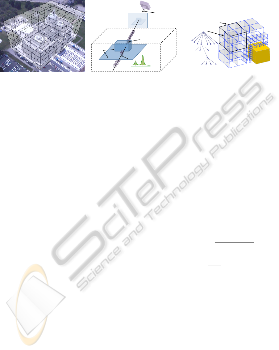
Figure 1: 1(a) and 1(b) PVM proposed by Pollard and Mundy (Pollard and Mundy, 2007; Pollard, 2008). 1(b) explains the

voxel notation, a pixel I

back projects into a ray of voxels R

, V is the unique voxel along R

that produces the intensity I

1(c) Octree subdivision of space proposed by Crispell (Crispell, 2010).

erywhere in space, and that are learned in unre-

stricted settings from images sequences.

2. To characterize for the ﬁrst time the local, 3-d

information in the PVM. The result are novel,

view-invariant, volumetric features that describe

local neighborhoods of the probabilistic informa-

tion of 3-d surface geometry and appearance in

the scenes.

3. A demonstration of the descriptive power, through

rigorous analysis of function approximation and

object recognition experiments, of features based

on a Taylor series approximation, and PCA analy-

sis of the probabilistic information in the models.

Encouraging initial recognition results promise

successful extensions based on generalization

of 2-d features e.g. Harris corners (Harris and

Stephens, 1988), HOG (Dalal and Triggs, 2005),

SIFT (Lowe, 2004), and 3-d differential features

(Sipiran and Bustos, 2010; Raviv et al., 2010), to

the probabilistic models in question.

4. The creation of the largest database of probabilis-

tic volume models available today.

The rest of the paper is organized as follows: Sec-

tion 1.1 explains the probabilistic volume model used

to learn the 18 areal sites of the city of Providence

used in this work. Section 2 discusses two types of

features used to model local neighborhoods in the vol-

umetric scenes. Section 3 explains category learning

and object classiﬁcation. Section 4 presents the exper-

imental results. Finally, conclusions and further work

are described in Sections 5 and 6.

1.1 Probabilistic Volume Model

Pollard and Mundy (2007) proposed a probabilistic

volume model that can represent the ambiguity and

uncertainty in 3-d models derived from multiple im-

age views. In Pollard’s model (Pollard and Mundy,

2007; Pollard, 2008), a region of three-dimensional

space is decomposed into a regular 3-d grid of cells,

called voxels (See Figure 1). A voxel stores two kinds

of state information: (i) the probability that the voxel

contains a surface element and (ii) a mixture of Gaus-

sians that models the surface appearance of the voxel

as learned from a sequence of images. The surface

probability is updated by incremental Bayesian learn-

ing (see Equation 1 below), where the probability of

a voxel X containing a surface element after N+1 im-

ages increases if the Gaussian mixture (see Equation 2

below) at that voxel explains the intensity observed in

the N+1 image better than any other voxel along the

projection ray. The resulting models look more like

volumetric models obtained from CT scans than mod-

els obtained from point clouds generated by range

scanners (see Figure 2).

N+1

(X ∈ S) = P

(X ∈ S)

N+1

|X ∈ S)

N+1

)

(1)

p(I) =

∑

k=1





2πσ

exp

−

(I−µ

)

2σ





(2)

In a ﬁxed-grid voxel representation, most of the

voxels may correspond to empty areas of a scene,

making storage of large, high-resolution scenes pro-

hibitively expensive. Crispell (2010) proposed a con-

tinuously varying probabilistic scene model that gen-

eralizes the discrete model proposed by Pollard and

Mundy. Crispell’s model allows non-uniform sam-

pling of the volume leading to an octree representa-

tion that is more space-efﬁcient and can handle ﬁner

resolution required near 3-d surfaces, see Figure 1(c).

The octree representation (Crispell, 2010), makes

it feasible to store models of large urban areas. How-

ever, learning times of large scenes using the PVM

remained impractical until recently, when a GPU im-

plementation was developed by Miller et al. (2011).

ICPRAM 2012 - International Conference on Pattern Recognition Applications and Methods

182

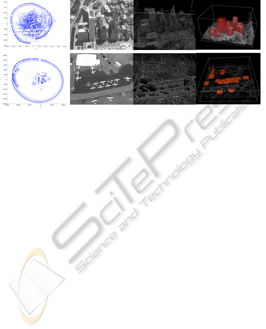
Figure 2: From left to right (column by column): Camera path and 3-d points (only used for visualization purposes) obtained

using Bundler (Snavely and Seitz, 2006). Details of collected video frames. The learned expected appearance volumes, EVM.

Examples of bounding boxes around objects of interest (this ﬁgure is best seen in color).

Training times decrease by several orders of magni-

tudes, depending on available computing resources

and model complexity, see (Miller et al., 2011) for

performance comparisons evaluated on single core

CPU and OpenCL implementation on CPU and GPU.

With a GPU framework in place is now feasible to

think of multi-class object recognition tasks where

large number of objects are required for training.

2 VIEW INDEPENDENT 3-D

FEATURES

This section describes how the geometry and appear-

ance information at every voxel are used to compute

a voxel’s expected appearance. It then describes two

approaches used to characterize the local information

(i.e. expected appearances) in the volumetric scenes,

namely PCA features and Taylor features.

2.1 Expected Volume Model

Though the work by Pollard was designed to de-

tect changes in a new image, the occupancy and ap-

pearance information can be used to render synthetic

images of the expected scene appearance (Pollard,

2008). For every pixel in the image, its intensity

is the summation, across all voxels in its projection

ray, of the expected color of the voxel and the likeli-

hood of that voxel containing a surface element and it

not being occluded. Consider a pixel I

, which back

projects into a ray of voxels R

, if V is the unique

voxel along R

that causes the intensity value at the

pixel, then the expected intensity at I

is explained by

(3) and (4) (also see Figure 1(b)).

E(I

) =

∑

∈R

E(I

|V = X

)P(V = X

) (3)

∑

∈R

E(I

|V = X

)P(X

∈ S)P(X

is not occluded) (4)

E(I

|V = X

) represents the expected intensity,

given that voxel X

∈ R

produced the intensity seen

in the image. This quantity is obtained from the mix-

ture of Gaussians stored at voxel X

. P(X

∈ S) is

the probability of X

containing a surface element

and it is also stored at X

. P(X

is not occluded) is

deﬁned as the probability that all voxels (along R

)

between X

and the camera contain empty space i.e.

P(X

is not occluded) =

∏

(1 − P(X

∈ S)).

For every ray containing a particular voxel

, the quantity E(I

|V = X

)P(X

∈ S) remains

unchanged, and the only ray-dependent term is

P(X

is not occluded). When learning neighborhood

conﬁgurations in the PVM, only the ray-independent

information is taken into account. The information at

every voxel is combined into to the quantity in Equa-

tion (5) (see below), here referred to as a voxel’s ex-

pected appearance, and the volume of expected ap-

pearances, as the expectation volume model, EVM.

E(I

|V = X

)P(X

∈ S) (5)

2.2 PCA Features

One way to represent the volumetric model is by iden-

tifying local spatial conﬁgurations that account for

OBJECT RECOGNITION IN PROBABILISTIC 3-D VOLUMETRIC SCENES

183

most of the variation in the data. Principal Com-

ponent Analysis (PCA) is carried out to ﬁnd the or-

thonormal basis that represents the volumetric sam-

ples in the best mean squared error sense. The prin-

cipal components are arranged in decreasing order of

variation as given by the eigenvalues of the sample

scatter matrix.

In order to perform PCA, feature vectors are ob-

tained by sampling locations on the scene according

to the octree structure, i.e. ﬁne sampling in regions

near surfaces and sparse sampling of empty space.

At each sampled location, n

l × n

l cubical re-

gions are extracted (centered at the sampled location),

where

l is the length of the smallest voxel present in

the 3-d scene. The extracted regions are arranged into

vectors by traversing the space at a resolution of

l, and

using a raster visitation schedule.

The scatter matrix S, of randomly sampled vec-

tors, is updated using a parallel scheme (Chan et al.,

1979) to speed up computation, and the principal

components are found by the eigenvalue decompo-

sition of S. In the PCA space, every neighborhood

(represented by a d-dimensional feature vector x) can

be exactly expressed as x =

x +

∑

i=1

, where e

are principal axes associated with the d eigenval-

ues, and a

are the corresponding coefﬁcients. A k-

dimensional (k < d) approximation of the neighbor-

hoods can be obtained by using the ﬁrst k principal

components i.e.

x =

x +

∑

i=1

. Section 4 presents

a detailed analysis of the reconstruction error of lo-

cal neighborhoods, namely |x −

, as a function of

dimension and training set size. In the remainder of

this paper, the vector arrangement of projection coef-

ﬁcients in the PCA space is referred as a PCA feature.

2.3 Taylor Features

Mathematically, the appearance function in the scene

can be approximated (locally) by its Taylor series ex-

pansion. The computation of derivatives in the ex-

pectation volume model, EVM, can be expressed as

a least square error minimization of the following en-

ergy function.

E =

∑

i=−ni

n j

∑

j=−n j

∑

k=−nk



V (i, j, k) −

V (i, j, k)



(6)

Where

V (i, j, k) is the Taylor series approxima-

tion of the expected 3-d appearance of a volume V

centered on the 3-d point (i, j, k). Using the second

degree Taylor expansion of V about (0, 0, 0), (6) be-

comes

E =

∑



V (x) −V

− x

G −



(7)

Where V

, G, H are the zeroth derivative, the gra-

dient vector and the Hessian matrix of the volume

of expected 3-d appearance about the point (0, 0, 0),

respectively. The coefﬁcients for 3-d derivative op-

erators can be found by minimizing (7) with re-

spect to the zeroth, ﬁrst and second order deriva-

tives. The computed derivative operators are applied

algebraically to neighborhoods in the EVM. The re-

sponses to the 10 Taylor operators, which correspond

to the magnitude of the zeroth, ﬁrst and second order

derivatives, are arranged into 10-dimensional vectors

and are referred to as Taylor features.

3 3-D OBJECT LEARNING AND

RECOGNITION

This section explains in detail the model used to learn

ﬁve object categories. It is important to keep in mind

that models are based on either Taylor features of

PCA features, but not both. The results obtained for

the two representations are presented in Section 4.

3.1 The Model: Bag of Features

Bag-of-features models have their origins in texture

recognition (Varma and Zisserman, 2009; Leung and

Malik, 1999) and bag-of-word representations for text

categorization (Joachims, 1997). Their application

to categorization of visual data is very popular in

the computer vision community (Sivic et al., 2005;

Csurka et al., 2004) and have produced impressive

results in benchmark databases (Zhang et al., 2007).

The independence assumptions inherent to bag-of-

features representation make learning models for few

object categories a simple task, assuming enough

training samples are available to learn the classiﬁca-

tion space. In this paper, a bag-of-features represen-

tation is constructed for ﬁve categories as outlined in

the following subsections.

3.2 Learning a Visual Vocabulary with

k-means

In order to produce a ﬁnite dictionary of 3-d expected

appearance patterns, the scenes are represented by a

set of descriptors (Taylor or PCA) that are quantized

using k-means-type clustering. Two major limitations

of k-means clustering must be overcome: (i) the algo-

rithm does not determine the best number of means,

i.e k, and (ii) it converges to a local minimum that

may not represent the optimum placement of cluster

centers.

ICPRAM 2012 - International Conference on Pattern Recognition Applications and Methods

184

To address (i), there exist available algorithms to

automatically determine the number of clusters (Pel-

leg and Moore, 2000; Hamerly and Elkan, 2003).

However, in the experiments in this paper the algo-

rithm was run using various values of k. An op-

timal value was selected based on object classiﬁca-

tion performance and running times. Disadvantage

(ii) requires careful attention because the success of

k-means depends substantially on the starting posi-

tions of the means. In the experiments, the train-

ing scenes are represented by millions of descriptors

(even if only a percentage of them are used), and ran-

dom sampling of k means, where k << 1 × 10

, may

not provide a good representation of the 3-d appear-

ance patterns.

The means are initialized using the algorithm pro-

posed by Bradley and Fayyad (1998), which has been

shown to perform well for large data sets (Maitra

et al., 2010). In the initialization algorithm (Bradley

and Fayyad, 1998), a random set of sub-samples of

the data is chosen and clustered via modiﬁed k-means.

The clustering solutions are then clustered using clas-

sical k-means, and the solution that minimizes the

sum of square distances between the points and the

centers is chosen as the initial set of means. In or-

der to keep computation time manageable, while still

choosing an appropriate number of sub-samples (10

being suggested in (Maitra et al., 2010; Bradley and

Fayyad, 1998)), an accelerated k-means algorithm

(Elkan, 2003) is used whenever the classical k-means

procedure is required.

The large number of volumetric training features

can only be practically processed using parallel com-

putation. While parallel clustering algorithms are

available (Judd et al., 1998), message passing be-

tween iterations could not be easily implemented for

the current framework. Therefore, an approximate k-

means method was selected, which is a modiﬁcation

of the reﬁnement algorithm by Bradley and Fayyad

(1998). The modiﬁed k-means algorithm is the fol-

lowing:

1. Sample an initial set of means, SP, as described above

2. Divide training samples into J blocks. Let CM =

3. Process each block in parallel as follows:

a. Let S

be the data in block J

b. CM

= AcceleratedKMeans(SP, S

, K)

4. CM =

i=0

, FM =

5. Process each CM

in parallel as follows:

a. FM

= AcceleratedKMeans(CM

,CM, K)

6. FM = argmin

Distortion(FM

,CM)

The minimization function, Distortion(FM

,CM),

computes the sum of square distances of each data

point to its nearest mean (for all J estimates). The set

of clusters with the smallest distortion value is cho-

sen as the ﬁnal solution, FM. The proposed algorithm

does not seek to improve the complexity of the tradi-

tional k-means algorithm but to manage memory re-

quirements and allow parallel processing of large data

sets.

3.3 Learning and Classiﬁcation

With a 3-d appearance vocabulary in place, individual

objects are represented by feature vectors that arise

from the quantization of the PCA or Taylor descrip-

tors present in that object. These feature vectors can

be used in supervised multi-class learning, where a

naive Bayes classiﬁer is used for its simplicity and

speed. During learning, the classiﬁer is passed train-

ing objects used to adjust the decision boundaries;

during classiﬁcation, the class label with the maxi-

mum a posteriori probability is chosen to minimize

the probability of error.

Formally, let the objects of a particular category be

the set O

i=1

, where l is the class label and N

the number of objects with class label l. Then, the set

of all labeled objects is deﬁned as O =

l=1

, where

is the number of categories. Let the vocabulary of

3-d expected appearance patterns be deﬁned as V =

i=1

, where k is the number of cluster centers in

the vocabulary. From the quantization step a count is

obtained, c

i j

, of the number of times a cluster center,

, occurs in object o

. Using Bayes formula, the a

posteriori class probability is given by:

P(C

) ∝ P(o

)P(C

) (8)

The likelihood of an object is given by the product of

the likelihoods of the independent entries of the vo-

cabulary, P(v

), which are estimated during learn-

ing. The full expression for the class posterior be-

comes:

P(C

) ∝ P(C

)

∏

j=1

P(v

)

(9)

∝ P(C

)

∏

j=1







∑

m=1:o

∈O

∑

n=1

∑

m=1:o

∈O







(10)

According to the Bayes decision rule, every ob-

ject is assigned the label of the class with the largest

a posteriori probability. In practice, log likelihoods

were computed to avoid underﬂow of ﬂoating point

computations.

OBJECT RECOGNITION IN PROBABILISTIC 3-D VOLUMETRIC SCENES

185

(a) (b) (c)

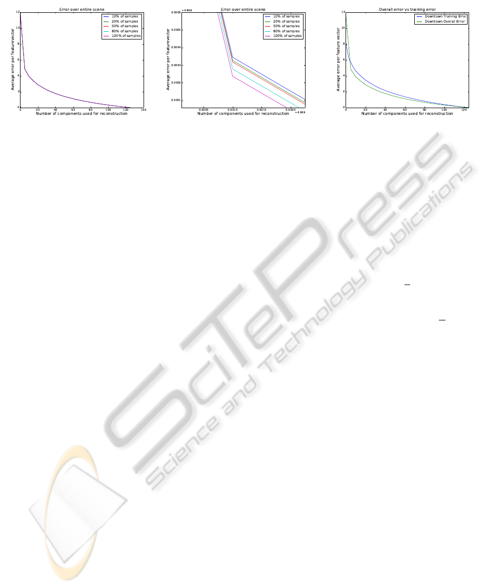
Figure 3: Analysis of reconstruction error. 3(a) Error as a function of the number of components used. The different curves

represent different proportion of samples used to perform PCA. 3(b) A zoomed-in detail of 3(a). 3(c) Comparison of errors

obtained over training neighborhoods vs. all available neighborhoods.

4 EXPERIMENTS AND RESULTS

The data collection and scene reconstruction pro-

cesses are now described, followed by comparisons

of scene data modeling accuracy based on either PCA

or Taylor features. The section concludes with multi-

class object recognition results, where objects from

8 scenes were classiﬁed among 5 categories; planes,

cars, houses, buildings, and parking lots. Training

samples consist of labeled objects from 10 scenes

(different from the ones used for testing). In order

to localize surface features through k-means, only

features centered at leaf-cells at the ﬁnest resolution

level of the octree were considered i.e. cells contain-

ing high occupancy probability

4.1 Data Collection and Scene

Formation

The aerial data used to build 18 different probabilis-

tic volume scenes was collected from a helicopter ﬂy-

ing over Providence, RI, USA, and its surroundings.

An approximate resolution of 30 cm/pixel was ob-

tained in the imagery and translated to 30 cm/voxel

in the models. The camera matrices for all image se-

quences were obtained using Bundler (Snavely and

Seitz, 2006). The probabilistic volume models were

learned using a GPU implementation (Miller et al.,

2011). For multi-class object recognition, bounding

boxes around objects of interest were given a class

label. Ten scenes were used for training and eight

for testing. Figure 2 contains examples of aerial im-

ages collected for these experiments, the EVMs and

the bounding boxes used to label objects of interest.

4.2 Neighborhood Reconstruction

Error

Ideally, the difference between the original expected

appearance data and the data approximated using

PCA or a Taylor series expansion should be small.

The difference between the reconstructed data and the

original data was measured as the average square dif-

ference between neighborhoods, i.e.

∑

train

i=1

|x −

where x and

x are the vector arrangement of the orig-

inal and the approximation neighborhoods, respec-

tively. For Taylor features,

x = V

+ x

G +

Hx.

For PCA features

x =

x +

∑

i=1

. In the experi-

ments, the size of the extracted neighborhoods was

l ×5

l being the length of the smallest voxel in

the model. The error was computed for the top scene

in Figure 2, here referred to as the Downtown scene.

Using all available neighborhoods to learn the

PCA basis is impractical; thus, a set of experiments

were performed to evaluate the reconstruction error

for different sizes of randomly chosen neighborhoods.

Figures 3(a) and 3(b) show the reconstruction error

for different sample sizes (as a percentage of the to-

tal number of neighborhoods). The error was basi-

cally identical for all computed fractions and 10%

was the fraction used for the remaining of the ex-

periments. Figure 3(c) compares the projection error

over the training samples and the overall projection

error (over all available neighborhoods). The curves

are very similar, indicating that the learned basis rep-

resents the training and testing data with compara-

ble accuracy. Finally, the reconstruction error for a

10-dimensional approximation in the PCA space was

compared to the reconstruction error achieved using a

-degree Taylor approximation. The results in Ta-

ble 1 indicate that a 2

-degree Taylor approximation

represents expected appearance of 3-d patterns with

only slight less accuracy than a PCA projection onto

a 10-dimensional space.

ICPRAM 2012 - International Conference on Pattern Recognition Applications and Methods

186

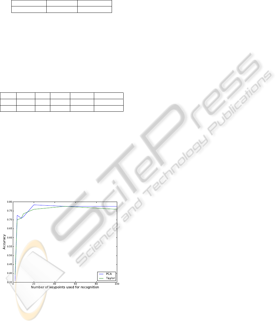
Table 1: Average approximation error over all 5x5x5 neigh-

borhoods. PCA and Taylor approximations are compared

for the Downtown scene.

Scene Name PCA Error Taylor Error

Downtown 3.88 4.05

4.3 3-d Object Recognition

This section presents multi-class object recognition

results. Five object categories were learned: planes,

cars, buildings, houses, and parking lots. Table 2

presents the number of objects in each category used

during training and classiﬁcation.

Table 2: Number of objects in every category.

Planes Cars Houses Buildings Parking Lots

Train 18 54 61 24 27

Test 16 29 45 15 17

Two measurements were used to evaluate the clas-

siﬁcation performance: (i) classiﬁer accuracy (i.e the

fraction of correctly classiﬁed objects), and (ii) the

confusion matrix. During classiﬁcation experiments,

the number of clusters in the codebook was varied

from k = 2 to k = 100. Figure 4 presents classiﬁcation

accuracy as a function of the number of clusters. For

both, Taylor-based features and PCA-based features,

the performance improves rapidly up to a 20-word

codebook, with little or no improvement for larger

vocabularies. Thus, for the remaining of the experi-

ments k was set to 20.

Figure 4: Classiﬁcation Accuracy. The curves represent the

fraction of correctly classiﬁed objects as a function of the

number of clusters.

Figure 5 presents examples of class distributions

learned with PCA and Taylor codebooks of twenty

features. To facilitate interpretation, the volumetric

form of the vocabulary entries are arranged along the

x-axis. It is important to keep in mind that each voxel

(in the volumetric feature), contains its expected 3-

d appearance as deﬁned by Eq. 5. The value of

expected 3-d appearance ranges from [0, 2] (and the

color used in the volumetric rendering from black to

white respectively). For empty space, the information

in the voxels is dominated by the occupancy proba-

bility, which takes values in the interval [0,1]; thus,

empty neighborhoods appear black. Appearance val-

ues, which are initially learned between [0,1], are off-

set to [1,2], to avoid confusing dark surfaces with

empty space. White voxels represent white surfaces

with a high occupancy probability; dark surfaces are

represented by gray voxels. For the planes cate-

gory, see Figures 5(a) and 5(c), empty neighborhoods,

white surface neighborhoods and neighborhoods con-

taining half white-surface space and half empty space

are the most common features. On the other hand, the

buildings category, see Figures 5(b) and 5(d), is rep-

resented by mid range neighborhoods corresponding

to dark surfaces and slowly changing derivatives.

Finally, the confusion matrices for a 20-keyword

vocabulary of PCA-based features and Taylor-based

features, are shown in Tables 6(a) and 6(b). Both

methods recognize planes, cars and parking lots with

high accuracy. Lower performance for buildings and

houses is expected, since a more discriminative model

is needed to successfully differentiate such similar

categories. The PCA-based representation is slightly

better at learning effective models for cars than the

Taylor based representation.

5 CONCLUSIONS

This paper presented a completely new representation

for object recognition models, where view-invariant

features were extracted directly from 3-d probabilis-

tic information. The representation was used to learn

and recognize objects from ﬁve different categories.

To the author’s knowledge, this work represents the

ﬁrst attempt to apply this representation to the classi-

ﬁcation of aerial scenes or indeed any type of scene.

The performance of the proposed features, was rig-

orously tested through reconstruction accuracy and

object categorization experiments. The recognition

results are very encouraging with high accuracy on

labeling bounded regions containing objects of the

selected categories. The experiments show that dif-

ferential geometry features derived from appearance

lead to essentially the same recognition performance

as PCA. This suggests that additional features repre-

senting geometric relationships deﬁned on differen-

tial geometry are likely to have good performance and

represent a basis for formally extending the feature

vocabulary.

OBJECT RECOGNITION IN PROBABILISTIC 3-D VOLUMETRIC SCENES

187

(a) Plane - PCA (b) Building - PCA

Figure 5: Class histograms for plane and building categories. The top row corresponds to class representations learned

with PCA-based features. The bottom row corresponds to those learned with Taylor-based features. The x-axis shows the

volumetric form of the 20 features; the y-axis, the probability of each feature. The most probable volumetric features for each

class are shown beside each histogram.

True

Class

Plane

House

Building

Car

Parking

Lot

Plane

House

Building

Car

Parking

Lot

0.86

0.02

0.00

0.03

0.00

0.67

0.27

0.00

0.12

0.00

0.31

0.67

0.00

0.07

0.93

0.00

0.14

0.00

0.03

0.88

(a) PCA

True

Class

Plane

House

Building

Car

Parking

Lot

Plane

House

Building

Car

Parking

Lot

0.86

0.02

0.00

0.03

0.00

0.64

0.27

0.00

0.12

0.00

0.33

0.67

0.00

0.07

0.86

0.00

0.14

0.00

0.10

0.88

(b) Taylor

Figure 6: Confusion matrix for a 20-keyword codebook of

PCA based features on the left and Taylor based features on

the right.

While there are many computational and storage

challenges faced when learning multiple object cate-

gories in large volumetric scenes, the work presented

in this paper makes an important contribution towards

true 3-d, view-independent object recognition. The

object categorization results demonstrate the descrip-

tive power of the PVM for 3-d object recognition and

open an avenue to more complex recognition systems

for dense, 3-d probabilistic scenes.

6 FURTHER WORK

The current feature representation will be extended to

incorporate features detected with differential opera-

tors that have been used successfully in 2-d featured-

based recognition systems and 3-d object retrieval al-

gorithms, e.g. 2-d and 3-d features based on the Har-

ris operator (Harris and Stephens, 1988; Sipiran and

Bustos, 2010), 3-d heat kernels based on the Laplace-

Beltrami operator (Raviv et al., 2010), SIFT features

(Lowe, 2004), HOG features (Dalal and Triggs, 2005)

and others. The occlusion, shadows and 3-d relief

present in the imagery collected for the experiments

presented in this work, pose great challenges to 2-d

multi-view recognition systems. However, in future

work, it will prove informative to compare 2-d multi-

view systems to the framework presented in this pa-

per.

The probabilistic scenes learned for this work

have known orientation and scale. In order to keep

feature-base representation of objects compact, future

work will explore representations for scale-invariant

and isometric features. Localization of objects is also

a desirable goal for future algorithms.

Finally, more advanced recognition models should

make full use of the geometric relations inherent

in the probabilistic volume model. Compositional

recognition models could represent a venue to learn

and share parts, allowing for object representations

that are efﬁcient, discriminative and geometrically co-

herent.

ICPRAM 2012 - International Conference on Pattern Recognition Applications and Methods

188

REFERENCES

Bariya, P. and Nishino, K. (2010). Scale-Hierarchical 3D

Object Recognition in Cluttered Scenes. IEEE Con-

ference on Computer Vision and Pattern Recognition.

Bradley, P. S. and Fayyad, U. M. (1998). Reﬁning Initial

Points for K-Means Clustering. In Proceedings of the

15th International Conference on Machine Learning.

Bronstein, A. M., Broinstein, M. M., Guibas, L. J., and Ovs-

janikov, M. (2011). Shape Google: Geometric Words

and Expressions for Invariant Shape Retrieval. ACM

Transactions on Graphics.

Chan, T. F., Golub, G. H., and LeVeque, R. J. (1979). Up-

dating Formulae and a Pairwise Algorithm for Com-

puting Sample Variances. Technical report, Depart-

ment of Computer Science. Stanford University.

Crispell, D., Mundy, J., and Taubin, G. (2008). Parallax-

Free Registration of Aerial Video. In BMVC.

Crispell, D. E. (2010). A Continuous Probabilistic Scene

Model for Aerial Imagery. PhD thesis, School of En-

gineering, Brown University.

Csurka, G., Dance, C. R., Fan, L., Willamowski, J., and

Bray, C. (2004). Visual categorization with bags of

keypoints. In In Workshop on Statistical Learning in

Computer Vision, ECCV.

Dalal, N. and Triggs, B. (2005). Histograms of oriented

gradients for human detection. In IEEE Conference

on Computer Vision and Pattern Recognition.

Drost, B., Ulrich, M., Navab, N., and Ilic, S. (2010). Model

Globally, Match Locally: Efﬁcient and Robust 3D Ob-

ject Recognition. IEEE Conference on Computer Vi-

sion and Pattern Recognition.

Elkan, C. (2003). Using the triangle inequality to acceler-

ate k-means. In Proceedings of the Twentieth Interna-

tional Conference on Machine Learning.

Felzenszwalb, P., McAllester, D., and Ramanan, D. (2008).

A discriminatively trained, multiscale, deformable

part model. In IEEE Conference on Computer Vision

and Pattern Recognition.

Fergus, R., Perona, P., and Zisserman, A. (2003). Ob-

ject class recognition by unsupervised scale-invariant

learning. In IEEE Conference on Computer Vision and

Pattern Recognition.

Freeman, W. and Adelson, E. (1991). The design and use of

steerable ﬁlters. IEEE Transactions on Pattern Analy-

sis and Machine Intelligence.

Gupta, P., Arrabolu, S., Brown, M., and Savarese, S. (2009).

Video scene categorization by 3D hierarchical his-

togram matching. In International Conference on

Computer Vision.

Hamerly, G. and Elkan, C. (2003). Learning the k in k-

means. In Seventeenth annual conference on neural

information processing systems (NIPS).

Harris, C. and Stephens, M. (1988). A combined corner and

edge detector. Alvey vision conference.

Joachims, T. (1997). Text Categorization with Support Vec-

tor Machines: Learning with Many Relevant Features.

In ECML.

Judd, D., McKinley, P., and Jain, A. (1998). Large-scale

parallel data clustering. IEEE Transactions on Pattern

Analysis and Machine Intelligence.

Leung, T. and Malik, J. (1999). Recognizing surfaces us-

ing three-dimensional texton. In Proceedings of the

Seventh IEEE International Conference on Computer

Vision.

Lowe, D. G. (2004). Distinctive Image Features from Scale-

Invariant Keypoints. International Journal of Com-

puter Vision.

Maitra, R., Peterson, A. D., and Ghosh, A. P. (2010). A sys-

tematic evaluation of different methods for initializing

the K-means clustering algorithm. In IEEE Transac-

tions of Knowledge and Data Engineering.

Miller, A., Jain, V., and Mundy, J. (2011). Real-time Ren-

dering and Dynamic Updating of 3-d Volumetric Data.

In Proceedings of the Fourth Workshop on General

Purpose Processing on Graphics Processing Units.

Mundy, J. L. and Ozcanli, O. C. (2009). Uncertain geom-

etry: a new approach to modeling for recognition. In

2009 SPIE Defense, Security and Sensing Conference.

Ozcanli, O. and Mundy, J. (2010). Vehicle Recognition as

Changes in Satellite Imagery. In International Con-

ference on Pattern Recognition.

Papadakis, P., Pratikakis, I., and Theoharis, T. (2010).

PANORAMA: A 3D Shape Descriptor Based on

Panoramic Views for Unsupervised 3D Object Re-

trieval. International Journal of Computer Vision.

Pelleg, D. and Moore, A. (2000). X-means: Extending K-

means with E cient Estimation of the Number of Clus-

ters. In International Conference on Machine Learn-

ing.

Pollard, T. (2008). Comprehensive 3-d Change Detection

Using Volumetric Appearance Modeling. PhD thesis,

Division of Applied Mathematics, Brown University.

Pollard, T. and Mundy, J. (2007). Change Detection in a 3-d

World. In IEEE Conference on Computer Vision and

Pattern Recognition.

Raviv, D., Bronstein, M. M., Bronstein, A. M., and Kim-

mel, R. (2010). Volumetric heat kernel signatures. In

3DOR ’10: Proceedings of the ACM workshop on 3D

object retrieval.

Shapira, L., Shalom, S., Shamir, A., Cohen-Or, D., and

Zhang, H. (2010). Contextual Part Analogies in 3D

Objects. International Journal of Computer Vision.

Sipiran, I. and Bustos, B. (2010). A Robust 3D Interest

Points Detector Based on Harris Operator. In Euro-

graphics Workshop on 3D Object Retrieval.

Sivic, J., Russell, B., Efros, A., Zisserman, A., and Free-

man, W. (2005). Discovering objects and their loca-

tion in images. In International Conference on Com-

puter Vision.

Snavely, N. and Seitz, S. (2006). Photo tourism: exploring

photo collections in 3D. ACM Transactions on Graph-

ics.

Thomas, A., Ferrar, V., Leibe, B., Tuytelaars, T., Schiel, B.,

and Van Gool, L. (2006). Towards Multi-View Object

Class Detection. In IEEE Conference on Computer

Vision and Pattern Recognition.

Varma, M. and Zisserman, A. (2009). A Statistical Ap-

proach to Material Classiﬁcation Using Image Patch

Exemplars. IEEE Transactions on Pattern Analysis

and Machine Intelligence.

OBJECT RECOGNITION IN PROBABILISTIC 3-D VOLUMETRIC SCENES

189

Zhang, J., Marszalek, M., Lazebnik, S., and Schmid, C.

(2007). Local Features and Kernels for Classiﬁcation

of Texture and Object Categories: A Comprehensive

Study. Int. J. Comput. Vision.

ICPRAM 2012 - International Conference on Pattern Recognition Applications and Methods

190