
IMPROVING FEATURE LEVEL LIKELIHOODS
USING CLOUD FEATURES
Heydar Maboudi Afkham, Stefan Carlsson and Josephine Sullivan
Computer Vision and Active Perception Lab., KTH, Stockholm, Sweden
Keywords:
Feature inference, Latent models, Clustering.
Abstract:
The performance of many computer vision methods depends on the quality of the local features extracted
from the images. For most methods the local features are extracted independently of the task and they remain
constant through the whole process. To make features more dynamic and give models a choice in the features
they can use, this work introduces a set of intermediate features referred as cloud features. These features take
advantage of part-based models at the feature level by combining each extracted local feature with its close by
local feature creating a cloud of different representations for each local features. These representations capture
the local variations around the local feature. At classification time, the best possible representation is pulled
out of the cloud and used in the calculations. This selection is done based on several latent variables encoded
within the cloud features. The goal of this paper is to test how the cloud features can improve the feature level
likelihoods. The focus of the experiments of this paper is on feature level inference and showing how replacing
single features with equivalent cloud features improves the likelihoods obtained from them. The experiments
of this paper are conducted on several classes of MSRCv1 dataset.
1 INTRODUCTION
Local features are considered to be the building
blocks of many computer vision and machine learning
methods and their quality highly effects the method’s
outcome. There are many popular methods for ex-
tracting local features from images. Among them
one can name sift (Lowe, 2003), hog(Dalal and
Triggs, 2005) and haar(Viola and Jones, 2001) fea-
tures, which are widely used for object detection
and recognition (Felzenszwalb et al., 2010; Laptev,
2006) and texture features such as maximum re-
sponse filter-banks (Varma and Zisserman, 2002) and
MRF(Varma and Zisserman, 2003) which are used for
texture recognition and classification. For most meth-
ods feature extraction is done independently from the
method’s task. For example in a normal inference
problem a model tries to decide between two differ-
ent classes. Usually for both hypothesises the same
constant extracted feature value is fed to the model.
In other words once the features are extracted, they
remain constant through the whole process.
Computer vision methods deal with local features
in different ways. Some such as boosting based ob-
ject detectors (Laptev, 2006; Viola and Jones, 2001)
and markov random fields (Kumar and Hebert, 2006),
depend on how discriminative single features are and
some, such as bag-of-words (Savarese et al., 2006),
depend on groups of features seen in a specific region
on the image. For the methods that depend on the dis-
criminative values of local features the inference done
at the feature level plays a critical role in the outcome
of the method. Improving the quality of feature level
inference can highly improve the quality of the object
level inference done by most of the methods.
Many studies have shown that using higher order
statistics, ex. the joint relation between the features,
can highly improve the quality of the features. Cap-
turing joint relations is popular with the bag-of-words
methods (Liu et al., 2008; Ling and Soatto, 2007)
since they deals with modeling joint relation between
a finite number of data clusters. Unfortunately not
many studies have focused on modeling joint relations
in non-discretized data to create features that capture
joint relations. A recent study on this matter is done
by Morioka et al. (Morioka and Satoh, 2010). In their
study they introduced a mechanism for pairing two
raw feature vectors together and creating a Pairwise
Codebook by clustering these pairs. As shown in their
work the clusters produced using these joint features
are more informative than the clusters produced using
single features. The idea behind their work is similar
431
Maboudi Afkham H., Carlsson S. and Sullivan J. (2012).
IMPROVING FEATURE LEVEL LIKELIHOODS USING CLOUD FEATURES.
In Proceedings of the 1st International Conference on Pattern Recognition Applications and Methods, pages 431-437
DOI: 10.5220/0003777904310437
Copyright
c
SciTePress
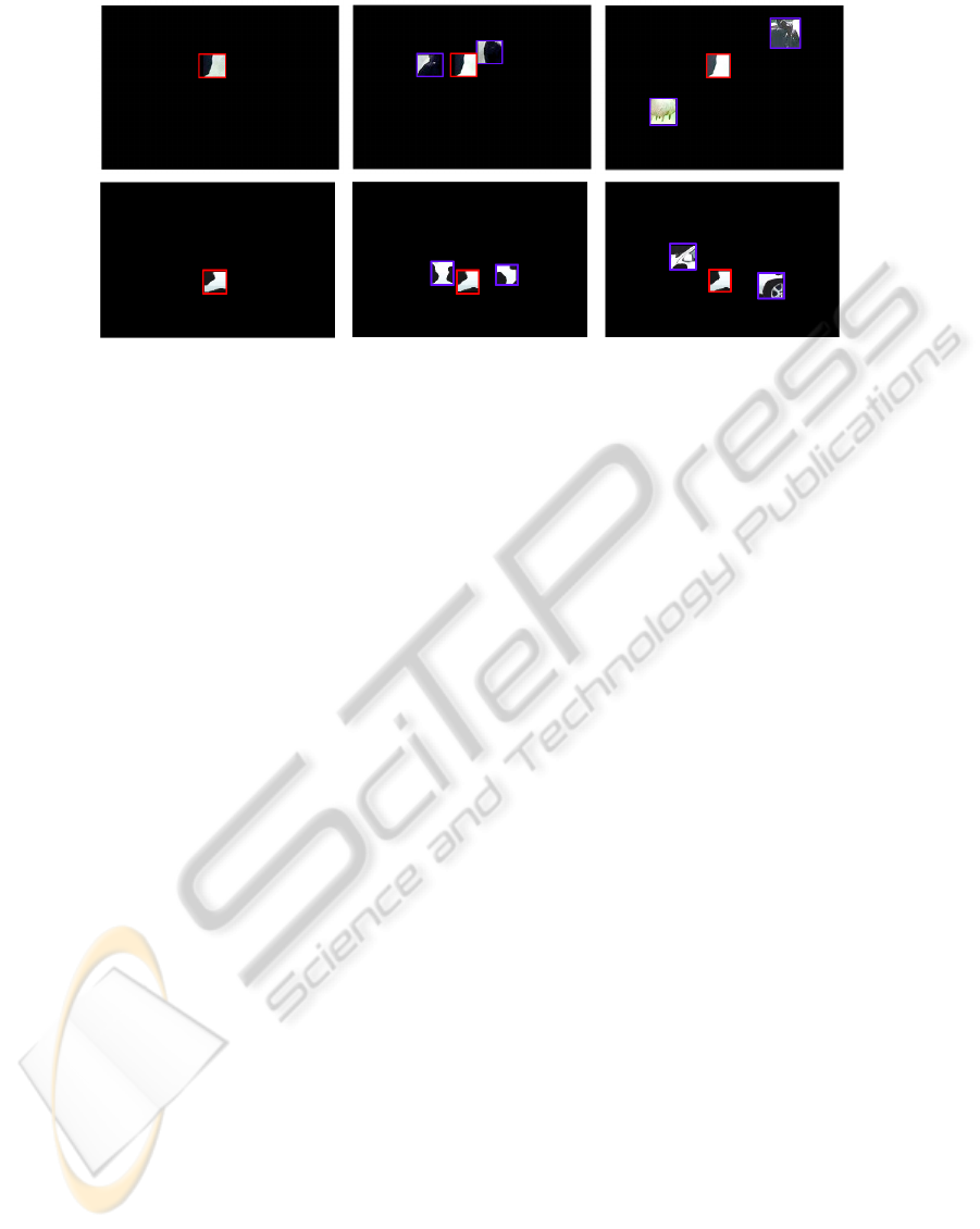
Figure 1: This figure gives an example of how local features are seen by a computer and how the neighbouring local features
can help with their inference. Here the task is to determine which object category of a certain feature. (Left Column)
The local feature is selected in both images. Clearly the information in this patch is not enough for determining the object
category.(Middle Column) By looking at the local features around the red patch (blue patches) more information is obtained.
This information supports the hypothesis of the red patch belonging to the cow object class in both images.(Right Column)
Taking another look around the red patch provides additional information. While in the first row this information supports
the previous observation, in the second row this information votes for the hypothesis of the patch belonging to the car object
class.
to the work in this paper while the methodology of
this work does not limit the number of feature vectors
used in creating more complex features.
The focus of this paper is solely on discriminative
analysis of the local features inference. For better un-
derstanding of the problem being solved in this paper,
the discussions are started with and example. Figure
1 helps with looking at the local features from a com-
puter’s point of view. Here the task is to determine to
which object category the red patch belongs to. This
figure shows how the joint information around a patch
can be used for extracting information regarding dif-
ferent hypothesises from the image data. This extrac-
tion can be misleading at some points but can lead
to an accurate solution in the long run. The method
introduced in this paper takes a similar approach to
this example to analyze the feature level likelihoods
in support of different hypothesises. Since such anal-
ysis can benefit many different methods, the analysis
is kept at the local feature inference. Here the assump-
tion is that a set of features are extracted from the im-
age and a relation is known between them that can
be captured by a graph. For example the features can
come from several patches within the image and their
spatial relation can be presented as a graph. These
features can be extracted using any feature extraction
method. The basic idea behind this paper is to use
the features and their relations to introduce a new set
of dynamic and changeable intermediate features in
terms of latent variables. These intermediate features
will be referred as cloud features. The latent variables
enable the feature to change its representation in dif-
ferent scenarios and their value is determined by an
optimization procedure to make it more discrimina-
tive for learning algorithms. This dynamic property of
cloud features provides a good ground for introducing
more discriminative features than the ones previously
extracted from the image.
The outline of this paper is as follow. The related
works to this paper are discussed in section 2. The
cloud features are discussed in detail in sections 3, 4
and 5. Finally section 6 discusses the behaviour of the
cloud features in some different scenarios.
2 RELATED WORKS
The goal of this paper is to present a method that takes
advantage of part-based models at the feature level to
come up with a set of intermediate features with dis-
criminative properties. In this section a brief review of
part based methods is provided and their differences
with the method presented in this paper is pointed out.
Later an example of studies that show how local fea-
tures can effect the overall inference is discussed.
Part-based models have been widely used in ob-
ject detection applications. A good example of such
application can be found in the work of Felzenszwalb
et al.(Felzenszwalb et al., 2009). These models con-
sist of a fixed root feature and several part feature with
their position as latent variables in relation to the root
feature. The part features are learnt either using ex-
ICPRAM 2012 - International Conference on Pattern Recognition Applications and Methods
432

(v
1
,φ
v1
)
(v
2
,φ
v2
)
(v
3
,φ
v3
)
(v
4
,φ
v4
)
(v
5
,φ
v5
)
(v
6
,φ
v6
)
(v
7
,φ
v7
)
(v
8
,φ
v8
)
(u, φ
u
)
F
u
z
1
f
�
z
1
z
2
f
�
z
2
Figure 2: (Left) A node u (a patch from an image) is connected to its neighboring nodes (close by patches). Here tree
node are selected (red patches) as a latent configuration. The quantitative value of this configuration is calculated as
(φ
u
,φ
v
2
,φ
v
5
,φ
v
7
).(Right) For any given point z in the feature space the closest vector within F
u
is selected as f
?
z
through
an optimization process. This shows how z can influence the value of F
u
.
act annotation (Felzenszwalb and Huttenlocher, 2005)
or as the result of an optimization problem (Felzen-
szwalb et al., 2009). Because of this latency the model
can have many configurations an usually the best con-
figuration is chosen among many due to the task in
hand. In these models the part features are used to
estimate a better confidence for the root feature.
Taking the part-based models to the feature level
comes with several difficulties. To begin with there
is larger variation at the feature level compared to the
object level. Here each local feature can play the role
of a root feature and completely different features can
be equally good representatives for the object class.
As an example consider the features obtained from
the wheel and the door of a car, one wishes for a car
model to return a high likelihood for both features de-
spite their differences. Also there is no right or wrong
way to look at local features. In this work the root
features and their parts are calculated as the result of
a clustering process. Since there is no best configura-
tion for these features each root feature can have sev-
eral good part configurations. These configurations
will capture the local variation around the local fea-
ture and will later be used for training non-linear dis-
criminative classifiers.
As mentioned in section 1 many methods benefit
from discriminative behaviours of local features. A
good example of such benefit can be seen in (Kumar
and Hebert, 2006) where the authors Sanjiv Kumar
et al. show how replacing generative models with
discriminative models benefits the MRF solvers and
improves their final results. Similar examples can
be widely found in numerous computer vision stud-
ies. The key difference between these works and this
method is the fact the features can change their value
to result in a more discriminative behaviour.
3 CLOUD FEATURES
To define the cloud features, let G(V, E) be a graph
with the extracted features as its nodes and the rela-
tion between them encoded as its edges. Also for each
node, say u, let φ
u
denote the feature vector associated
to this node and N
u
denote the its neighbors. A cloud
feature, with its root at node u and m latent parts, is
the set of all possible vectors that are created by con-
catenating the feature vector of node u and the feature
vectors of m nodes selected from N
u
. This set is for-
mally defined as
F
u
= {(φ
u
,φ
v
1
,...,φ
v
m
)|v
i
∈ N
u
}, (1)
where (φ
u
,φ
v
1
,...,φ
v
m
) is the concatenation of the fea-
ture vector of the nodes u,v
1
,...,v
m
. In other words all
possible configurations that can be made using u and
its parts exist in the set F
u
. This can also be seen as the
space of all variations around node u. These config-
urations are shown in figure 2 (Left). In this figure a
node u (a patch extracted from an image) is connected
to its neighbours (its close by patches). In the shown
configuration three neighbors v
2
,v
5
,v
7
are selected
shown using solid line edges. The resulting feature
vector for this configuration is (φ
u
,φ
v
2
,φ
v
5
,φ
v
7
). Here
the set F
u
will contain all possible similar feature vec-
tors made by selecting three nodes among the eight
neighbors.
In practice only one of the vectors within F
u
is
selected and used as its quantitative value. Since the
size set of this can grow large this value is selected in
an optimization process. This value is determined in
relation to a fixed target point in the feature space. For
any arbitrary point z in the feature space, the value of
F
u
is fixed as the best fitting vector in F
u
to this point.
This can be written as
f
?
z
= argmin
f ∈F
u
{d( f ,z)}. (2)
IMPROVING FEATURE LEVEL LIKELIHOODS USING CLOUD FEATURES
433

Here d(.) is a metric distance. Here the point z is
used as an anchor point in the feature space for fixing
latent variables of the cloud feature. Figure 2 (Right)
illustrates how f
?
z
is selected. In this work z plays an
important role in the classification process. Since for
every given z the value of F
u
changes, z can be seen
as a tool for pulling out different properties of F
u
. In
the classification stage each F
u
will be fit to different
z values, learnt during the training process, to verify
whether F
u
contains configurations that belong to the
object or not.
By having a prior knowledge of how the nodes are
distributed in N
u
a partitioning can be imposed on this
set. This partitioning will later be referred as the ar-
chitecture of the cloud feature. This partitioning is
designed in a way that each latent part comes from
one partition. This partitioning can slightly reduce
the complexity of the optimization.
Efficient solving of the optimization problem 2
can have a large effect on the performance and the
running time of the methods using cloud features. As-
suming that the size of the extracted features is fixed
and distance is measured using euclidean distance, the
complexity of implemented method is calculated as
O(|N
u
|m), where is m is the number of latent parts.
By introducing an architecture and partitioning N
u
,
this complexity will be reduced to O(|N
u
|). In other
words this problem can be solved by visiting the
neighbors of each node at most m times. It is pos-
sible to design more efficient algorithms for solving
this optimization problem and this will be in the fo-
cus of the future works of this paper.
4 LATENT CLASSIFIERS
In this problem the task of a classifier is to take
a cloud feature and classify it to either being from
the object or not. For a set of labeled features,
{(F
u
1
,y
1
),.. ., (F
u
N
,y
N
)} gathered from the training
set, the goal is to design a function c that uses one or
several configurations within cloud features to mini-
mize the cost function
N
∑
i=1
|c(F
u
i
) − y
i
|. (3)
A key difference between this approach and other
available approaches is the fact that the local varia-
tions around the local feature are also modeled with
optimization of c. This means that not only the model
uses the value of the root feature but it also uses the
dominant features appearing around the root feature
regardless of their spatial position.
The optimization problem 3 is approximated by
defining the function c as a linear basis regression
function with model parameters z
1
,z
2
,...,z
M
,W . The
values z
1
,z
2
,...,z
M
are M anchor points in the feature
space for fixing the latent variables capturing different
configurations of the features and W = (w
0
,...,w
M
)
contains the regression weights, these parameters are
learnt during the training stage. Using these parame-
ters, the regression function c is defined as
c(F
u
;z
1
,.. ., z
M
,W ) =
M
∑
m=1
w
m
Φ
z
m
(F
u
) + w
0
. (4)
Here the basis function Φ
z
m
measures how good F
u
can be fit to z
m
. This basis function can be written
as any basis function for example a Gaussian basis
function is defined as
Φ
z
m
(F
u
;s) = exp(−
d( f
?
z
m
,z
m
)
2
2s
2
). (5)
Equations 4 and 5 clearly show that the decision made
for F
u
depend both on the different values in F
u
and
how good it can be fit to z
m
values. Due to the dy-
namic section, F
u
can be fit to different z
m
values
which makes the scoring processes harder for neg-
ative samples. Solving equation 4 to obtain W is
straight forward once the z
m
values are known.
The local features come from different regions of
an object and these regions are no visually similar.
This fact results in a large variation on the data used
for training. This variation can not be captured by
only one set of M configurations. To solve this prob-
lem a mixture model of K sets each with M different
configurations is considered and each set is associated
with a different regression model. When classifying a
cloud feature, it is initially assigned to the model that
minimizes the over all fitting cost, defined as
argmin
k∈{1...K}
{
M
∑
m=1
d( f
?
z
(k)
m
,z
(k)
m
)}. (6)
Here the model is chosen based on how good the fea-
ture F
u
is fit to all the configurations within the model.
5 LEARNING THE PARAMETERS
The goal of the learning algorithms is to determine
the K configurations sets together with the regres-
sion function. It is possible to design an optimization
method to estimate all configurations together with
the regression function, but such optimization is more
suitable for an object level classification since the data
contains less variation at that level. In this work the
optimization is done two separate steps. The first step
ICPRAM 2012 - International Conference on Pattern Recognition Applications and Methods
434
x
y
scale
x
y
scale
x
y
scale
x
y
scale
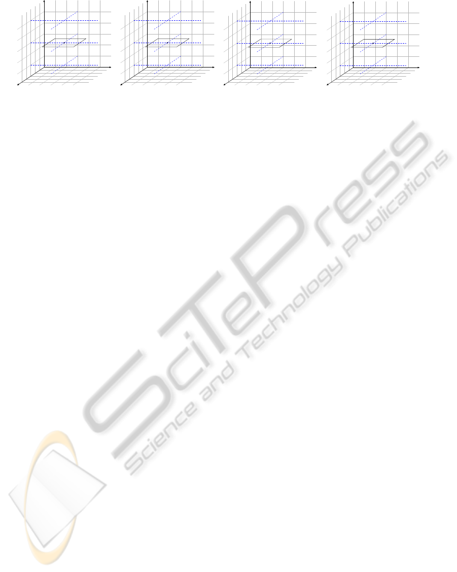
Figure 3: (Left) The Arc1 only depends on the patch itself. (Middle) The Arc2 Depends on the central patch together with
a selection of patches in the scale below (Details) the central patch. (Right) The Arc4 Depends on the central patch and a
selection of patches from from the scale level below (Details) and the scale level above (Context) the central patch.
uses a generative method for finding the K sets of con-
figurations. This generative method is an adaptation
k-means algorithm with the cost function
argmin
S
K
∑
k=1
∑
F
u
∈S
k
M
∑
m=1
d( f
?
z
(k)
m
,z
(k)
m
)
!
. (7)
This adaptation of k-means divides the features into
K clusters and the elements of each cluster have a
strong connection by sharing the M different config-
urations. This optimization can be solved using iter-
ative methods used for solving the k-means problem.
This method will be referred as L-KMEANS(K,M).
To determine the parameters initially L-
KMEANS(K,M) procedure is ran over the positive
features. This way the strong configurations ap-
pearing in the training set are formulated in terms
of cluster centers resulted by the procedure. These
cluster centers can be used for labeling all features.
For each cluster the variations in the negative features
is captured by running L-KMEANS(1,M) on the neg-
ative features assigned to that cluster. Finally, after
identifying both positive and negative configurations,
these configurations are used to fix the values of
cloud features and the and regression function 4 is
optimized to separate the positive features from the
negative features.
6 EXPERIMENTS AND RESULTS
The experiments conducted in this paper are not de-
signed to be compared with state of the art object de-
tectors but to test the hypothesis proposed in the pa-
per. The main idea behind the experiments is to eval-
uate the local features with different architectures and
compare them with the baseline which only contains
the root feature. The evaluation is straight forward,
each feature is scored using the equations 4 and 6 and
the results are presented in terms of different preci-
sion recall curves. The experiments are conducted on
several classes of MSRCv1 (Winn et al., 2005) dataset.
Several parameters control the behaviour of the
cloud features. As mentioned in section 3 the archi-
tecture of the cloud features imposes a strong prior on
how the latent parts are placed together. The architec-
ture controls the complexity of the feature by control-
ling the number of its latent parts. The flexibility of
these features is controlled by the number of neigh-
bors each node has in graph G. The larger the size of
the neighbours the wider the search space is for the
latent parts. The goal of the experiments to analyze
how the complexity and flexibility of the cloud fea-
tures effects their discriminative behavior. Unfortu-
nately, as the flexibility and the complexity of the fea-
tures increase the optimization processes in equations
7 and 4 become computationally expensive. There-
fore the results are only provided on a few classes of
this dataset.
The graph used in the experiments is build over
the fixed size patches with 30 pixel side extracted
from an image pyramid and described using a PHOG
descriptor (Bosch et al., 2007). The choice of this
graph is due to the future works of this paper when
these features are used to build object level classifiers.
Let G = (V,E) denote the graph built over the
patches extracted from the image pyramid with V
containing all extracted patches and for two patches
in V , say u and v, the edge uv belongs to E iff
|x
u
− x
v
| < t and |s
u
− s
v
| < 1. Here x
u
is the spatial
position, s
u
is the scale level of node u and t is a given
threshold which controls how patches are connected
to each other.
In this work four different architectures are con-
sidered. These architectures are considered as prior
information and are hard coded in the method. Al-
though it is possible to learn the architectures, learn-
ing them requires more tools which are not in the
scope of this paper. As mentioned in section 3 the
architecture is imposed by partitioning the set N
u
. In
this problem the neighbors of each node come from
three different scale levels. There are, of course, many
different ways that this set can be partitioned into m
subsets. To reduce the number of possibilities only
IMPROVING FEATURE LEVEL LIKELIHOODS USING CLOUD FEATURES
435
0 0.1 0.2 0.3 0.4 0.5 0.6 0.7 0.8 0.9 1
0
0.1
0.2
0.3
0.4
0.5
0.6
0.7
0.8
0.9
1
Recall
Precision
Car
( 0 − 0.5 )
( 0 − 1.0 )
( 0 − 2.0 )
( 0 − 3.0 )
( 1 − 0.5 )
( 1 − 1.0 )
( 1 − 2.0 )
( 1 − 3.0 )
( 2 − 0.5 )
( 2 − 1.0 )
( 2 − 2.0 )
( 2 − 3.0 )
( 3 − 0.5 )
( 3 − 1.0 )
( 3 − 2.0 )
( 3 − 3.0 )
0 0.1 0.2 0.3 0.4 0.5 0.6 0.7 0.8 0.9 1
0
0.1
0.2
0.3
0.4
0.5
0.6
0.7
0.8
0.9
1
Recall
Precision
Face
( 0 − 0.5 )
( 0 − 1.0 )
( 0 − 2.0 )
( 0 − 3.0 )
( 1 − 0.5 )
( 1 − 1.0 )
( 1 − 2.0 )
( 1 − 3.0 )
( 2 − 0.5 )
( 2 − 1.0 )
( 2 − 2.0 )
( 2 − 3.0 )
( 3 − 0.5 )
( 3 − 1.0 )
( 3 − 2.0 )
( 3 − 3.0 )
0 0.1 0.2 0.3 0.4 0.5 0.6 0.7 0.8 0.9 1
0
0.1
0.2
0.3
0.4
0.5
0.6
0.7
0.8
0.9
1
Recall
Precision
Plane
( 0 − 0.5 )
( 0 − 1.0 )
( 0 − 2.0 )
( 0 − 3.0 )
( 1 − 0.5 )
( 1 − 1.0 )
( 1 − 2.0 )
( 1 − 3.0 )
( 2 − 0.5 )
( 2 − 1.0 )
( 2 − 2.0 )
( 2 − 3.0 )
( 3 − 0.5 )
( 3 − 1.0 )
( 3 − 2.0 )
( 3 − 3.0 )
0 0.1 0.2 0.3 0.4 0.5 0.6 0.7 0.8 0.9 1
0
0.1
0.2
0.3
0.4
0.5
0.6
0.7
0.8
0.9
1
Recall
Precision
Cow
( 0 − 0.5 )
( 0 − 1.0 )
( 0 − 2.0 )
( 0 − 3.0 )
( 1 − 0.5 )
( 1 − 1.0 )
( 1 − 2.0 )
( 1 − 3.0 )
( 2 − 0.5 )
( 2 − 1.0 )
( 2 − 2.0 )
( 2 − 3.0 )
( 3 − 0.5 )
( 3 − 1.0 )
( 3 − 2.0 )
( 3 − 3.0 )
0 0.1 0.2 0.3 0.4 0.5 0.6 0.7 0.8 0.9 1
0
0.1
0.2
0.3
0.4
0.5
0.6
0.7
0.8
0.9
1
Recall
Precision
Bike
( 0 − 0.5 )
( 0 − 1.0 )
( 0 − 2.0 )
( 0 − 3.0 )
( 1 − 0.5 )
( 1 − 1.0 )
( 1 − 2.0 )
( 1 − 3.0 )
( 2 − 0.5 )
( 2 − 1.0 )
( 2 − 2.0 )
( 2 − 3.0 )
( 3 − 0.5 )
( 3 − 1.0 )
( 3 − 2.0 )
( 3 − 3.0 )
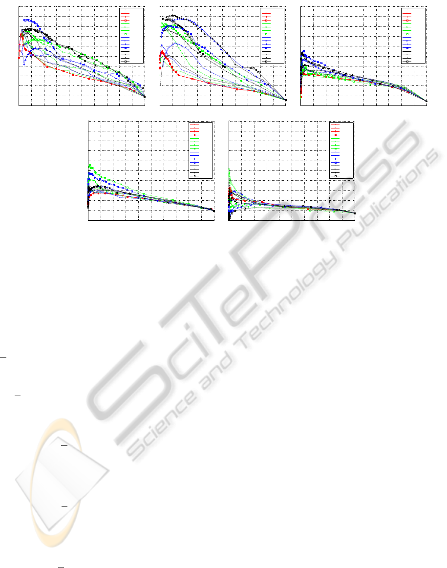
Figure 4: Results from the MSRCv1 dataset. Five classes {car,face,plane,cow,bike} were considered from this dataset. In this
experiment the value of t controlling number of neighbors was varied from the value equal to half the patch size to three times
larger than the patch size.
partitions with simple fixed scale and spatial relations
to the central node are considered. Twelve subsets are
formed by dividing the nodes (patches) in each scale
into four quadrants. The scale levels and quadrants
can be seen in the features shown in figure 3. A num-
ber of these subsets are selected to form different fea-
tures architectures. Let this selection be denoted by
P
u
. Using a subset of the twelve partitions, the four
architectures defined in this figure are,
• Arc 1: This architecture is created by having
P
u
=
/
0. This architecture uses the descriptor of the
central node as the descriptor. This feature will be
used as a benchmark for analyzing dynamic archi-
tectures.
• Arc 2: Let P
u
partition the scale level below the
scale level of u into four spatial quadrants. This
architecture contains the data from node u and ad-
ditional information about the details in this re-
gion.
• Arc 3: Let P
u
partition the scale level above the
scale level of u into four spatial quadrants. This
architecture contains the data from node u and ad-
ditional information about the context in this re-
gion.
• Arc 4: Let P
u
partition the scale levels both above
and below the scale level of u. This architecture
contains the data from u together with information
about details and the context of the region u has
appeared in.
Here each node can be described using each of the
four architectures and the goal is to verify the most
suitable architecture for the object region. To train
the classifiers any feature from the positive regions is
considered positive and the rest of the extracted fea-
tures are considered as negative features. This should
be kept in mind that the problem being solved here is
equivalent taking an arbitrary patch from an arbitrary
scale and location and asking whether it belongs to
the object or not. Due to the noise at the feature level
this problem is a hard problem to solve by nature.
Classes {Car,Face,Plane,Cow,Bike} are chosen
from this dataset. In this experiment all four archi-
tectures are used with varying t value to increase the
flexibility of features. . Here 256 models are used and
each with 5 positive and 5 negative latent configura-
tions. The results of this experiment can be seen in
figure 4. These experiments reveal several properties
about the cloud features. The first property is in fact
that the improvement obtained on the feature likeli-
hood level depend on both the base feature and the
architecture. At it can be seen in this figure the base
feature (red curves) has an easier time capturing the
properties of the car and face classes in comparison
with the rest of the classes. Also between these two
classes the architectures have an easier time capturing
the relations in face region. Meanwhile it is clearly
visible that for the bike class both the features and ar-
ICPRAM 2012 - International Conference on Pattern Recognition Applications and Methods
436

chitectures are failing to capture the local properties.
This figure also shows that there is no best architec-
ture for the all the object classes and the choice of the
architecture is completely object dependent. This can
be seen in the likelihoods obtained from the plane and
the cow classes, where the base likelihoods are similar
but the responses obtained from the different architec-
tures are different.
7 CONCLUSIONS AND FUTURE
WORKS
The main objective of this work has been to investi-
gate the improvement in discriminability obtained by
substituting simple local features with local adaptive
composite hierarchical structures that are computed at
recognition time from a set of potential structures de-
noted as ”cloud features”. This is motivated by the
fact that even at local feature level, intra class object
variation is very large, implying that generic single
feature classifiers that try to capture this variation will
be very difficult to design. In our approach this diffi-
culty is circumvented by the introduction of the cloud
features that capture the intra class variation an fea-
ture level. The price paid is of course a more com-
plex process for the extraction of local features that
are computed in an optimization process in order to
yield maximally efficient features. We believe how-
ever that this process can be made efficient by consid-
ering the dependencies and similarities between local
feature variations that are induced by the global intra
class object variation.
There are many ways to improve the performance
and accuracy of the cloud features and investigate
their applications. As mentioned in the text, coming
up with better optimization algorithms will decrease
the usage cost of these features. Meanwhile design-
ing algorithms for learning the architecture rather than
hard-coding them will increase the accuracy of these
features. As for the applications, these features can
be used in different object detection and recognition
platforms. A direct follow up of this work is using
these features to build more robust object detectors
for detecting object classes. Since the cloud features
are results of clustering process rather than discrimi-
native analysis, they can also be used in bag-of-words
models and will result in more discriminative words
and smoothed labeled regions.
ACKNOWLEDGEMENTS
This work was supported by The Swedish Foundation
for Strategic Research in the project Wearable Visual
Information Systems.
REFERENCES
Bosch, A., Zisserman, A., and Munoz, X. (2007). Repre-
senting shape with a spatial pyramid kernel. In CIVR,
pages 401–408. Association for Computing Machin-
ery.
Dalal, N. and Triggs, B. (2005). Histograms of oriented
gradients for human detection. In CVPR, pages 886–
893.
Felzenszwalb, P., Girshick, R., Mcallester, D., and Ra-
manan, D. (2009). Object detection with discrimina-
tively trained part based models. Pattern Analysis and
Machine Intelligence, IEEE Transactions on.
Felzenszwalb, P. F., Girshick, R. B., McAllester, D., and
Ramanan, D. (2010). Object detection with discrim-
inatively trained part-based models. IEEE Transac-
tions on Pattern Analysis and Machine Intelligence,
32:1627–1645.
Felzenszwalb, P. F. and Huttenlocher, D. P. (2005). Pictorial
structures for object recognition. IJCV, 61:55–79.
Kumar, S. and Hebert, M. (2006). Discriminative random
fields. IJCV, 68:179–201.
Laptev, I. (2006). Improvements of object detection using
boosted histograms. In BMVC, pages 949–958.
Ling, H. and Soatto, S. (2007). Proximity distribution ker-
nels for geometric context in category recognition. In
ICCV.
Liu, D., Hua, G., Viola, P., and Chen, T. (2008). Integrated
feature selection and higher-order spatial feature ex-
traction for object categorization. CVPR, 0:1–8.
Lowe, D. G. (2003). Distinctive image features from scale-
invariant keypoints.
Morioka, N. and Satoh, S. (2010). Building compact local
pairwise codebook with joint feature space clustering.
In ECCV, page 14, Crete, Greece.
Savarese, S., Winn, J., and Criminisi, A. (2006). Discrimi-
native object class models of appearance and shape by
correlatons. CVPR, 2:2033–2040.
Varma, M. and Zisserman, A. (2002). Classifying images of
materials: Achieving viewpoint and illumination in-
dependence. In ECCV, pages 255–271, London, UK.
Springer-Verlag.
Varma, M. and Zisserman, A. (2003). Texture classification:
Are filter banks necessary. In CVPR.
Viola, P. and Jones, M. (2001). Rapid object detection using
a boosted cascade of simple features. CVPR, 1:511.
Winn, J., Criminisi, A., and Minka, T. (2005). Object cat-
egorization by learned universal visual dictionary. In
ICCV, ICCV ’05, pages 1800–1807, Washington, DC,
USA. IEEE Computer Society.
IMPROVING FEATURE LEVEL LIKELIHOODS USING CLOUD FEATURES
437
