
BROADCAST NEWS PHONEME RECOGNITION
BY SPARSE CODING
Joseph Razik
1
, S´ebastien Paris
2
and Herv´e Glotin
1
1
LSIS/DYNI, Universit´e du Sud Toulon-Var, Avenue de l’Universit´e - BP20132, 83957 La Garde Cedex, France
2
LSIS/DYNI, Universit´e Aix-Marseille, Domaine universitaire de Saint J´erˆome, Avenue Escadrille Normandie Niemen,
13397 Marseille Cedex 20, France
Keywords:
MFCC, GMM, Sparse coding, Large-scale SVM, Explicit feature maps.
Abstract:
We present in this paper a novel approach for the phoneme recognition task that we want to extend to an
automatic speech recognition system (ASR). Usual ASR systems are based on a GMM-HMM combination
that represents a fully generative approach. Current discriminative methods are not tractable in large scale
data set case, especially with non-linear kernel. In our system, we introduce a new scheme using jointly
sparse coding and an approximation additive kernel for fast SVM training for phoneme recognition. Thus, on
a broadcast news corpus, our system outperforms the use of GMMs by around 2.5% and is computationally
linear to the number of samples.
1 INTRODUCTION
In recent years major advancements have been
achieved in speech processing. However, robust
speech recognition still remains a challenging task.
Current systems are still exhibiting difficulties when
dealing with real-life conditions such as: multiple-
speakers without training, noise, background music,
spontaneous speech. The most common architecture
of an automatic speech recognition (ASR) system is
based on a generative framework and more specially
a GMM-HMM approach (Gaussian Mixture Model -
Hidden Markov Model). Prior to fully decoding sen-
tences, a kind of phoneme recognition module is the
first and most crucial part of the ASR system.
The latter is usually modeled by a GMM with a
given number of components, large enough to capture
the intra-variability of the phonemes (Huang et al.,
2001). It assumes that the conditional pdf to each
phoneme’s class has a parametric form and that is
comprised a mixture of normal pdfs. In practice, this
strong assumption is mainly verified when training
data is sufficiently available, but can introduce some
over-fitting for less populated classes.
Recently, in vision systems, discriminative ap-
proaches combining bag-of-features and large-scale
classifiers have shown dramatic improvement versus
generative methods (Yang et al., 2009). These new
approaches relie on three basic ingredients: (i) an un-
supervised data encoding, (ii) feature extraction from
a learned dictionary with pooling, and (iii) fast SVM
(Support Vector Machines) for classification.
For the first step, sparse learning (see in (Lin et al.,
2008; Hsieh et al., 2008; Wang et al., 2010; Smit and
Barnard, 2009; Sivaram et al., 2010; Mairal et al.,
2010)) allows a smaller re-construction error with few
basis vectors, involving discriminative vectors’ dic-
tionary properties. After applying sparse code pool-
ing, we obtain features descriptors with only positive
or null values. In this case, specialized kernels such
as intersection histogram kernel, offer the state of the
art classification performances (Maji et al., 2009). In
(Vedaldi and Zisserman, 2011), such kernels can be
efficiently approximated via the feature map frame-
work, involving fast training (linear in number of
training samples (Fan et al., 2008)).
In this paper, we propose a new phoneme recogni-
tion system based on MFCC (Mel Frequency Cepstral
Coefficient) sparse coding and fast non-linear train-
ing.
First, in section 2 we will describe the audio
MFCC parameters as our input features, then in sec-
tion 3 we present a short overview of the GMM. Sec-
tion 4 provides an introduction of the sparse coding
framework. Pooling methods are presented in section
5. The large-scale linear SVM is reviewed in section
6 with also the feature maps homogeneous additive
kernel approximation method. Finally, sections 7 and
191
Razik J., Paris S. and Glotin H. (2012).
BROADCAST NEWS PHONEME RECOGNITION BY SPARSE CODING.
In Proceedings of the 1st International Conference on Pattern Recognition Applications and Methods, pages 191-197
DOI: 10.5220/0003778201910197
Copyright
c
SciTePress

8 are dedicated to corpus presentation and results.
2 PARAMETERS
The parameters extracted from the audio signal are
based on MFCC (Mel Frequency Cepstral Coeffi-
cients) (Davis and Mermelstein, 1980; Rabiner and
Juang, 1993) with CMS (Cepstral Mean Subtraction)
normalization. The frame-shift for their computation
is 10 ms.
Additionally to the static MFCC coefficients (C
0
...C
12
), we compute also dynamic information val-
ues as their first derivative and variance. More pre-
cisely, we compute and concatenate to the final pa-
rameter vector the variance, and several approximated
derivative coefficients according to the ranges be-
tween points for this calculation (20, 62, 125 and 250
ms). The usual approximation at time t is done by re-
gression with coefficients at t − α and t + α (Young
et al., 1995). Moreover, two size of the analysis win-
dow is used for the computation of the MFCC (16
and 32 ms). Thus, the final parameter vector is the
concatenation of each kind of parametrization and its
total dimension is 260, 13 statics and 13 dynamics by
5 kinds of dynamic coefficients and 2 window sizes.
2.1 Whitening
Several pre-processing methods of the parameter vec-
tors could be applied in order to have the data better
conditioned. The first simple pre-processing step is
to center the data, i.e. to make the mean of the pa-
rameter vector equals zero. In fact, the static MFCC
coefficients are already computed as centered with the
CMS normalization but the dynamic coefficients are
not.
In a second step, the entire data set of the vec-
tors may be whitened. This process is commonly
used in deep learning domain but not so frequently
in speech recognition (Ranzato et al., 2010). The
whitening process consists in decorrelating the data
and making their variances equal to unity by the use
of an eigen-value decomposition (EVD) (Hyv¨arinen
and Oja, 2000).
More precisely, if we called X the set of parameter
vectors, X is then linearly transformed into a whiten
set
˜
X with the property that E{
˜
X
˜
X
T
} = Id, the iden-
tity matrix. By using an EVD decomposition of the
preceding covariance matrix, we obtain the relation
E{
˜
X
˜
X
T
} = E∆E
T
, where E is the orthogonal matrix
of eigenvectors of E{
˜
X
˜
X
T
} and ∆ is the diagonal ma-
trix of its eigenvalues: ∆ = diag(δ
1
,.. ., δ
n
). The es-
timation of the whiten vectors ˜x can now be obtained
by the following equation:
˜x = E∆
−1/2
E
T
x (1)
where ∆
−1/2
= diag(δ
−1/2
1
,.. .,δ
−1/2
n
).
Thus, besides the raw parameter vectors we assess
the use of a whitening process on our MFCC data and
the impact on the recognition rate.
3 BASELINE SYSTEM: GMM
We compare our phoneme recognition method to one
based on Gaussian Mixture Models (GMM) that is
considered as a reference system in phoneme recog-
nition task.
GMMs are used as a generative classifier model-
ing data classes as a mixture of M Gaussian pdfs and
expressed as:
G(x|y;θ) =
M
∑
i=1
w
i
N (x,µ
i
,Σ
i
),
M
∑
i=1
w
i
= 1 (2)
for which, with vectors of n dimensions, the continu-
ous pdf is defined as:
N (x,µ,Σ) ,
1
p
(2π)
n
det(Σ)
exp(−
1
2
(x−µ)
T
Σ
−1
(x−µ)).
(3)
The w
i
coefficients represent the weights of
each Gaussian pdf composing the conditional pdf
G(x|y;θ). For each class y = j, j = 1, .. .,V, the
training process consists in learning parameters θ
j
,
{w
j,i
,µ
j,i
,Σ
j,i
}, i = 1,.. .,M by an EM algorithm
(Huang et al., 2001) and particularly with the HTK
software (Young et al., 1995). Moreover, to avoid
over-fitting we assume during the GMMs training that
the covariances matrices Σ
j,i
are diagonals and we
add an extra regularization term. For all the V = 41
classes, we will learn the conditional pdf G(x|y;θ)
by varying the number of components that maximizes
the accuracy, from M = 1 to M = 256.
4 FROM VECTOR
QUANTIFICATION TO SPARSE
CODING
Super-vectors coupled with a supervised training al-
gorithm represents a promising discriminating ap-
proach (Arous and Ellouze, 2003; Tomi Kinnunen,
2010). We propose to build such super-vectors us-
ing sparse coding and a pooling procedure. Let X
ICPRAM 2012 - International Conference on Pattern Recognition Applications and Methods
192

be the set of n × N-dimensional MFCC matrix ex-
tracted from the audio, i.e. X , [x
1
,.. .,x
N
] ∈ R
n×N
.
Let D be a dictionary made of K vectors such D ,
[d
1
,.. .,d
K
] ∈ R
n×K
and trained from data. This dic-
tionary clusters/resumes all data X into K codebook
vectors.
From this trained D, in the traditional vector quan-
tization (VQ) approach, each vector x
i
of X is as-
signed to only one d
j
such that:
d
j
= argmin
k=1,...,K
kx
i
− d
k
k
2
(4)
Let be C = [c
1
,.. .,c
K
] ∈ R
n×K
the VQ matrix for
which each c
i
vector has only one component c
j
i
6= 0
(corresponding to the d
j
codebook vector from the
preceding equation (4). The associated VQ optimiza-
tion problem is formulated as follows:
argmin
D,C
N
∑
i=1
kx
i
− Dc
i
k
2
2
s.t. kc
i
k
ℓ
0
= 1,∀i (5)
where kxk
ℓ
0
designs the pseudo zero-norm, i.e. only
one element of x is equal to 1, others are set to 0. In
equation (5), D,C must be optimized jointly by the
Kmeans algorithm or variants for example.
In the sparse coding (SC) approach, the difference
is that each vector x
i
can be expressed as a linear com-
bination of the vectors of the dictionary D and not
only by one of it. Then, the problem to solve is ex-
tended as in the following equation:
argmin
D,C
N
∑
i=1
kx
i
− Dc
i
k
2
2
+ λkc
i
k
ℓ
1
s.t. kc
i
k
ℓ
1
= 1
(6)
The regularization term λ coupled with the ℓ
1
norm, as seen in the equation (6), ensures the spar-
sity of the optimized codes. Unfortunately, this joint
constrained optimization does not have a convex ex-
plicit formulation and the resolution is done in two
steps, repeated iteratively until convergence.
The first step consists in updating the current es-
timation of the dictionary
b
D
t+1
given current sparse
codes
b
C
t
via a block coordinate descent optimizer.
The second step consists in updating sparse codes
b
C
t+1
given the current dictionary
b
D
t+1
via a LASSO
algorithm (Mairal et al., 2009).
5 SPARSE CODES POOLING TO
CONSTRUCT A NEW AUDIO
DESCRIPTOR
Each phoneme realization p
i
, i = 1,. ..,P, where P
defines the total number of phonemes in the data set,
is associated with F
i
MFCC vectors x
l
, l = 1,.. .,F
i
(of dimension n = 260 and such that
P
∑
i=1
F
i
= N, the
total number of audio parameter vectors). In order
to construct the new proposed audio feature vector
z
i
= [z
1
,.. .,z
K
] for this phoneme, all associated sparse
codes {c
l
}, l = 1, .. .,F
i
are projected/pooled by one
of the two following methods:
• Mean pooling:
z
j
i
=
1
F
i
F
i
∑
l=1
|c
j
l
| (7)
• Max pooling:
z
j
i
= max(|c
j
1
|,.. ., |c
j
F
i
|) (8)
The set of the P features {z
i
} and their correspond-
ing label will be trained efficiently with a large-scale
linear SVM. Since sparse dictionary learning coupled
with max-pooling method produce almost perfectly
linear separable descriptors, a fast linear SVM solver
such as Liblinear is preferred. This approach can be
perceived discriminative since we don’t focus on the
data densities to classify, but only on the frontiers of
separation.
6 LARGE-SCALE LINEAR
SUPPORT-VECTOR MACHINE
Once the descriptors are computed, a large-scale lin-
ear SVM can be used as classifier. For training
the model efficiently, according to the Vapnik the-
ory (Vapnik, 1998), we aim to minimize the structural
error in order to generalize performances on unseen
data. This leads to find a binary classifier separating
classes based on the maximum margin principle. Sev-
eral algorithms exist that aim to find models maximiz-
ing such margins, for example neural networks with
Generalized Relevance Learning Vector Quantization
(GLRVQ) (Hammer et al., 2004), some variant of ad-
aboosting (Rudin et al., 2007) and the popular SVM
(Vapnik, 1998). A finer analysis indicates that the
second error term of the total risk’s upper bound is in-
creasing when the Vapnik-Chervonenkis (VC) dimen-
sion ~ is also increasing. This latter is directly linked
BROADCAST NEWS PHONEME RECOGNITION BY SPARSE CODING
193

with the particular choice of the kernel, ~ = 2K + 1
for linear kernel and ~ = ∞ for RBF kernel. In other
words, one may prefer a simple linear separator espe-
cially when the input feature dimension K is high. It
will generally perform close to those obtained with a
non-linear specialized kernel but with faster training
and prediction.
SVM is trained classically with the Sequential
Minimal Optimization (SMO) algorithm (Sch¨olkopf
et al., 2001) with a complexity O(KP
2
) where P is
the number of training examples (in the worst case,
when P
sv
= P, P
sv
is the number of support vectors).
This quadratic dependency from P can be reduced if
we particularize kernels to linear ones and by intro-
ducing an extra tolerance term ε in the minimization
problem. This leads to large-scale linear SVM solvers
based on efficient Newton optimizers (Hsieh et al.,
2008) or stochastic gradient descent (on the primal
form, see (Shalev-Shwartz et al., 2007)). Complexity
of such a large-scale solver is reduced to O(KP).
Let us define the set of sparse code descriptors
(after mean- or max-pooling) Z , {z
1
,.. .,z
P
} and
their corresponding labels y , {y
1
,.. .,y
P
} where z
i
∈
Z ⊆ R
K
and y
i
∈ {−1,1}. Thus, each phoneme
recognition is considered as a class/non-class prob-
lem with a one-against-all approach. P corresponds
to the number of phoneme realizations, which is in-
ferior to the total number N of MFCC parameter vec-
tors and equals the number of descriptors after pool-
ing method.
The linear SVM problem consists of finding the
hyperplane parameter bw minimizing the sum of a ℓ
2
loss function and a ℓ
2
regularization term such that:
bw
T
= argmin
w
(
1
2
w
T
w+C
M
∑
i=1
max
1− y
i
w
T
z
i
,0
2
)
(9)
To solve this problem, we use a modified version
of the liblinear 1.5 package (Fan et al., 2008) accept-
ing dense input vectors
1
. Any new input vector y
will be classified as bz = sign( f(z; bw)) = sign(bw
T
z) ∈
{−1, 1} by a simple scalar product in O(K).
6.1 Fast Non-linear Method for
Approximated Additive
Homogeneous Kernels via Explicit
Feature Maps
For linear SVM, evaluation is performed with a
simple scalar product f
l
(z;w) = w
T
z taking O(K)
1
Available at http://www.cs.berkeley.edu/?smaji/projects
/digits/.
whereas for non-linear kernel the expansion be-
comes f
nl
(z;β) =
P
sv
∑
i=1
β
i
K(z,z
i
) taking approximately
O(KP
sv
). Both for training and predicting, SVM with
non-linear kernels is at least P
sv
slower.
First introduced by (Maji et al., 2009) for the
intersection histogram (IH) kernel and extended to
any homogeneous additive kernels (IH, χ
2
, Shannon-
Jensen) in (Vedaldi and Zisserman, 2011), an ex-
plicit closed form of the feature maps associated to
these kernels, denoted Ψ(z), permits the approxima-
tion f
nl
(z) ≈ w
′T
Ψ(z) = w
′T
z
′
. Moreover the Ψ(z)
approximation is independent of the training data.
Now w
′
and z
′
∈ R
(2v+1)K
where v is the approxi-
mation order (typically v = {1,2}) and f
nl
(z) runs in
O((2v+ 1)K).
Assuming z
j
is the j
th
components of z, j =
1,.. .,K then for any homogeneous kernel, Ψ(z
j
) is
approximated as follows:
b
Ψ
i
(z
j
) =
p
b
κ
0
i = 0,
q
2z
j
b
κ
i+1
2
cos
i+1
2
Llogz
j
i > 0 odd,
q
2z
j
b
κ
i
2
sin
i
2
Llogz
j
i > 0 even,
(10)
b
κ
i
is the i
th
value of the spectrum κ(ω) sampled
with a sampling frequency equal to L. Closed forms
of κ(ω) depend on the chosen kernel type and read-
ers can retrieve details in (Vedaldi and Zisserman,
2011). For an efficient implementation, Vedaldi also
proposes to pre-compute values of
b
Ψ
i
(z
j
) for wide
dynamic of z
j
and store them in a table. With this
approach, retrieving
b
Ψ
i
(z
j
) with this given table runs
in O(2ν+ 1).
Since it takes an extra O((2v + 1)K) to compute
Ψ(z) from z, total run time for using an additive
homogeneous kernel is O(2(2v + 1)K) (Ψ(z)+f
nl
(z)
computation) and even more important is independent
of P
sv
and consequently of the training size P. The ac-
celeration is proportional to
P
nv
2(2v+1)
for the non-linear
case.
To make experimentations, we used a modifica-
tion of the Scenes/Objects Classification Matlab tool-
box framework which implements all the above men-
tioned processing (Paris, 2011).
7 CORPUS DESCRIPTION
To develop our method, we used about 2 hours of
French radio broadcast news. This corpus was ex-
tracted from a larger broadcast news corpus pro-
vided by the 2006 ESTER French evaluation cam-
ICPRAM 2012 - International Conference on Pattern Recognition Applications and Methods
194
paign (Gravier et al., 2004; Galliano et al., 2006;
Razik et al., 2011). This corpus contains only broad-
band speech (no narrow band, no music segments)
and sentence level transcriptions are provided. How-
ever, some sentences may have background noise or
music. There are 72 speakers in the 2 hours, 28 fe-
males and 44 males. This corpus is more difficult and
more realistic (noise, number of classes, etc.) than the
usual TIMIT data set.
In our study, we work at phoneme level, so we
used a forced alignment process of the data by exter-
nal acoustical models and lexicon of a large vocab-
ulary speech recognition systems (Illina et al., 2004).
We used a decomposition onV = 41 french phonemes
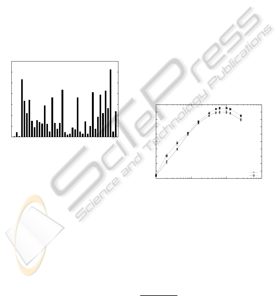
including silence and short pause. Figure 1 shows the
histogram of the phoneme distribution within the 2
hours of our corpus.
0
1000
2000
3000
4000
5000
6000
7000
sp
S
R_l
a
d
E
sil
j
Z
y
on
u
k
in
g
t
e
z_l
v
s
t_l
H
n_l
b
z
eh
w
euf
oh
eu
f
i
O
n
swa
m
l
p
R
o
an
# Occurrences
Phonemes
Figure 1: Phoneme distribution in the corpus.
As with this corpus some phonemes are underrep-
resented, we will use a cross validation technique in
10 subsets to assess the performance of both devel-
oped systems instead of fixed training, development
and test corpora. One of the ten subset was used as a
development corpus to tune the hyperparameter of the
SVM.
The subsets were not defined or clustered ac-
cording to the speakers thus forthcoming results are
speaker independent.
According to the corpora size, the different results
are given in recognition rate and standard deviation
(vertical bars in figures), and to a significance confi-
dence of around 0.2% at 0.95 level of significance.
8 RESULTS
As the corpus is labeled in 41 phoneme classes, we
learn 41 GMM models (one model for each phoneme)
with various number of components. We use the HTK
toolkit (Young et al., 1995) for extracting both the
MFCC coefficients and training the GMM models
2
.
We assess a number of Gaussian mixtures vary-
ing between 1 to 256. Figure 2 shows that the GMM
system obtained a best performance of about 61% of
accuracy for 100 mixtures on our corpus. This perfor-
mance is of good level knowing that our corpus can be
considered difficult (only 1h of training data, broad-
cast radio condition).
8.1 Whitening The Data
Additionally to the comparison between GMM and
SC/SVM model, we assess the use of a whitening pre-
processing of the MFCC data as explained in section
2.1.
Figure 2 shows the accuracy rate of the GMM
phoneme recognition system according to the number
of mixtures for both raw and whiten MFCC data. As
for the case of image processing (Coates et al., 2011),
whitening the data before computing both GMM or
Sparse Dictionary improves the results by around 1%
in absolute.
42
44
46
48
50
52
54
56
58
60
62
1 10 100 1000
Accuracy [%]
Number of mixtures
No Whitening
Whitening
Figure 2: Effect of whitening with GMM according to the
number of mixtures (log scale).
8.2 Sparse Coding/SVM
In the SC/SVM based system, we assess the role of
several parameters on the accuracy as the choice of
the pooling method, the use of linear or non-linear
kernel (intersection kernel) for the SVM and of course
the size of the dictionary.
Concerning the recognition system process, the
SVM hyper-parameter is tuned globally on all
phoneme classes and not specifically to each class.
Moreover, the descriptor vectors (sparse codes) are
2
However we do not use the Hidden Markov Model
(HMM) capability of HTK and trained our GMM by a one
state HMM.
BROADCAST NEWS PHONEME RECOGNITION BY SPARSE CODING
195
normalized according to the kernel type. In the linear
case, the vectors should be ℓ
2
normalized, and in the
non-linear case, the vectors should be ℓ
1
normalized
(Vedaldi and Zisserman, 2011).
In our experiment, the system obtains the same ac-
curacy performance whatever which pooling method
is used.
As we mentioned, the use of an approximated
non-linear kernel SVM improves the accuracy of our
system compared to the linear case. Figure 3 shows
the accuracy of both linear and intersection kernels.
We can note that the approximated non-linear system
performs better than the linear one. Even if their ac-
curacy are close, the difference between both is sig-
nificant and the training time is just slightly increased
by 2ν+ 1 where ν = 1 in our study.
44
46
48
50
52
54
56
58
60
62
64
10 100 1000 10000
Accuracy [%]
Dictionary size
approximated IH kernel
linear kernel
Figure 3: Accuracy with linear and approximated IH kernel
(ν = 1) in log scale.
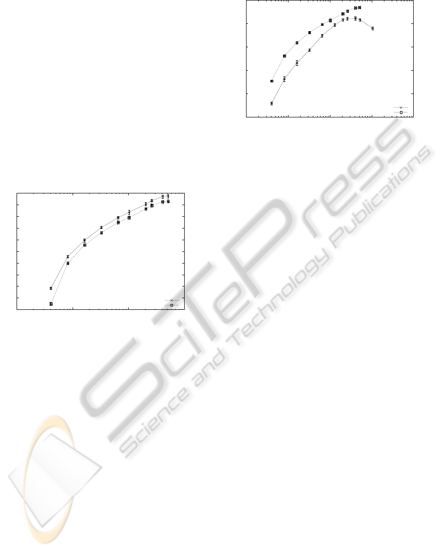
8.3 GMM vs. Sparse Coding
We compare both GMM and Sparse Coding based
systems on the corpus. In order to compare their re-
sults, we consider that a GMM with M mixtures is
similar to a codebook dictionary with K = 41 × M
vectors (number of classes by number of mixtures).
Figure 4 shows the accuracy of both system ac-
cording to this comparison scale. The SC/SVM
based system outperforms the GMM based system by
around 2.5% in absolute (63.5% for the Sparse Cod-
ing/SVM and 61.1% for the GMM) at their best.
9 CONCLUSIONS AND
PERSPECTIVES
In this paper we showed that the sparse coding ap-
proach outperforms significantly the classic GMM.
For any number of Gaussian components, the system
40
45
50
55
60
65
10 100 1000 10000 100000
Accuracy [%]
Dictionary size
GMM system
SC/SVM system
Figure 4: Accuracy of SC/SVM vs. GMM (log scale).
using the equivalent number of sparse codes outper-
forms the GMM. An advantage of the sparse coding
method is that it needs less training samples to learn
a representative dictionary and the representation is
more compact. The GMM method is more sensitive
to the total amount of available data and to the initial-
ization step. Moreover, in this paper we achieved re-
sults close to a specialized non-linear kernel thanks to
the additive homogeneous kernel approximation, still
linear in computation time.
Several directions could be explored to further im-
prove the performance of the sparse approach, includ-
ing Laplacian constraints in the sparse codes con-
struction to obtain a more reliable codebook versus
a slight change in the data (Wang et al., 2010), us-
ing a hierarchical construction of the codebook (Yu
et al., 2011), or providing a feature selection method
based on MKL (Multiple Kernel Learning) (see FGM
– Feature Generating Machine algorithm (Tan et al.,
2010)). Although we used an unsupervised method
for building the codebook, it is also possible to train
simultaneously the dictionary and the classifier in a
supervised way (Mairal et al., 2008).
Furthermore, the results obtained in this study are
only focused on the phone stage of speech recogni-
tion. We should evaluate the impact of the improve-
ment at this level on the final word recognition rate
of a complete ASR system. However, the ASR sys-
tem can still be based on an HMM classifier with the
observation matrix directly build with the probability
outputs of the SVM. It has the advantage of being a
method both generative and discriminative. Finally,
as it has been introduced more recently, it is possible
to use a structural SVM learning discriminately and
simultaneously the temporal structure and the sparse
codes in linear time (Joachims et al., 2009).
ICPRAM 2012 - International Conference on Pattern Recognition Applications and Methods
196

REFERENCES
Arous, N. and Ellouze, N. (2003). Cooperative supervised
and unsupervised learning algorithm for phoneme
recognition in continuous speech and speaker-
independent context. Neurocomputing, 51:225–235.
Coates, A., Lee, H., and Ng, A. Y. (2011). An analysis of
single-layer networks in unsupervised feature learn-
ing. In Artificial Intelligence and Statistics (AISTATS),
page 9.
Davis, S. and Mermelstein, P. (1980). Comparison of para-
metric representations for monosyllabic word recog-
nition in continuously spoken sentences. IEEE Trans.
ASSP, 28:357–366.
Fan, R.-E., Chang, K.-W., Hsieh, C.-J., Wang, X.-R., and
Lin, C.-J. (2008). LIBLINEAR: A library for large
linear classification. Journal of Machine Learning Re-
search, 9:1871–1874.
Galliano, S., Geoffrois, E., Gravier, G., Bonastre, J.,
Mostefa, D., and Choukri, K. (2006). Corpus descrip-
tion of the ester evaluation campaign for the rich tran-
scription of french broadcast news. In LREC, pages
315–320.
Gravier, G., Bonastre, J., Galliano, S., and Geoffrois, E.
(2004). The ester evaluation compaign of rich tran-
scription of french broadcast news. In LREC.
Hammer, B., Strickert, M., and Villmann, T. (2004). Rel-
evance lvq versus svm. In Artificial Intelligence and
Softcomputing, springer lecture notes in artificial in-
telligence, volume 3070, pages 592–597. Springer.
Hsieh, C.-J., Chang, K.-W., Lin, C.-J., and Keerthi, S. S.
(2008). A dual coordinate descent method for large-
scale linear svm.
Huang, X., Acero, A., and Hon, H. (2001). Spoken Lan-
guage Processing: A Guide to Theory, Algorithm and
System Development. Prentice Hall.
Hyv¨arinen, A. and Oja, E. (2000). Independent component
analysis: algorithms and applications. Neural Netw.,
13:411–430.
Illina, I., Fohr, D., Mella, O., and Cerisara, C. (2004). The
automatic news transcription system : Ants, some real
time experiments. In ICSLP, pages 377–380.
Joachims, T., Finley, T., and Yu, C.-N. (2009). Cutting-
plane training of structural svms. Machine learning,
77(1):27–59.
Lin, C.-J., Weng, R. C., and Keerthi, S. S. (2008). Trust
region newton method for logistic regression. J. Mach.
Learn. Res., 9.
Mairal, J., Bach, F., Ponce, J., and Sapiro, G. (2009). On-
line dictionary learning for sparse coding. In Proceed-
ings of the 26th Annual International Conference on
Machine Learning, ICML ’09, pages 689–696, New
York, NY, USA. ACM.
Mairal, J., Bach, F., Ponce, J., and Sapiro, G. (2010). On-
line learning for matrix factorization and sparse cod-
ing. Journal of Machine Learning Research, 11:19–
60.
Mairal, J., Bach, F., Ponce, J., Sapiro, G., and Zisserman,
A. (2008). Supervised dictionary learning. Advances
Neural Information Processing Systems, pages 1033–
1040.
Maji, S., Berg, A. C., and Malik, J. (2009). Classification
using intersection kernel support vector machines is
efficient. In CVPR.
Paris, S. (2011). Scenes/objects classification toolbox.
http://www.mathworks.com/matlabcentral/fileexchan
ge/29800-scenesobjects-classification-toolbox.
Rabiner, L. and Juang, B. (1993). Fundamentals of Speech
Recognition. Prentice Hall PTR.
Ranzato, M., Krizhevsky, A., and Hinton, G. (2010). Fac-
tored 3-way restricted boltzmann machines for mod-
eling natural images. In International Conference on
Artificial Intelligence and Statistics AISTATS.
Razik, J., Mella, O., Fohr, D., and Haton, J.-P. (2011).
Frame-synchronous and local confidence measures
for automatic speech recognition. IJPRAI, 25(2):157–
182.
Rudin, C., Schapire, R. E., and Daubechies, I. (2007). Anal-
ysis of boosting algorithms using the smooth margin
function. The Annals of Statistics, 35(6):2723–2768.
Sch¨olkopf, B., Platt, J. C., Shawe-Taylor, J. C., Smola, A. J.,
and Williamson, R. C. (2001). Estimating the support
of a high-dimensional distribution. Neural Comput.,
13:1443–1471.
Shalev-Shwartz, S., Singer, Y., Srebro, N., and Cotter, A.
(2007). Pegasos: Primal estimated sub-gradient solver
for svm.
Sivaram, G., Nemala, S., M. Elhilali, T. T., and Hermansky,
H. (2010). Sparse coding for speech recognition. In
ICASSP, pages 4346–4349.
Smit, W. J. and Barnard, E. (2009). Continuous speech
recognition with sparse coding. Computer Speech and
Language, 23:200–219.
Tan, M., Wang, L., and Tsang, I. W. (2010). Learning sparse
svm for feature selection on very high dimensional
datasets. In ICML, page 8.
Tomi Kinnunen, H. L. (2010). An overview of text-
independent speaker recognition: From features to su-
pervectors. Speech Communication, 52:12–40.
Vapnik, V. N. (1998). Statistical Learning Theory. Wiley-
Intersciences.
Vedaldi, A. and Zisserman, A. (2011). Efficient additive
kernels via explicit feature maps. IEEE PAMI.
Wang, J., Yang, J., Kai Yu, F. L., Huang, T., and Gong, Y.
(2010). Locality-constrained linear coding for image
classification. CVPR’10.
Yang, J., Yu, K., Gong, Y., and Huang, T. S. (2009). Lin-
ear spatial pyramid matching using sparse coding for
image classification. In CVPR.
Young, S., Evermann, G., Kershaw, D., Moore, G., Odell,
J., Ollason, D., Valtchev, V., and Woodland, P. (1995).
The HTK Book. Entropic Ltd., Cambridge, England.
Yu, K., Lin, Y., and Lafferty, J. (2011). Learning image
representations from the pixel level via hierarchical
sparse coding. In CVPR, pages 1713–1720.
BROADCAST NEWS PHONEME RECOGNITION BY SPARSE CODING
197
