COMPUTATION OF THE NORMALIZED COMPRESSION

DISTANCE OF DNA SEQUENCES USING A MIXTURE OF

FINITE-CONTEXT MODELS

Diogo Pratas, Armando J. Pinho and Sara P. Garcia

Signal Processing Lab, IEETA/DETI, University of Aveiro, 3810–193 Aveiro, Portugal

Keywords:

Normalized-compression distance, Finite-context models, Human chromosomal similarity.

Abstract:

A compression-based similarity measure assesses the similarity between two objects using the number of bits

needed to describe one of them when a description of the other is available. For being effective, these measures

have to rely on “normal” compression algorithms, roughly meaning that they have to be able to build an internal

model of the data being compressed. Often, we ﬁnd that good “normal” compression methods are slow and

those that are fast do not provide acceptable results. In this paper, we propose a method for measuring the

similarity of DNA sequences that balances these two goals. The method relies on a mixture of ﬁnite-context

models and is compared with other methods, including XM, the state-of-the-art DNA compression technique.

Moreover, we present a comprehensive study of the inter-chromosomal similarity of the human genome.

1 INTRODUCTION

The work of Solomonoff, Kolmogorov, Chaitin

and others (Solomonoff, 1964; Kolmogorov, 1965;

Chaitin, 1966) on how to measure complexity has

been of paramount importance for several areas of

knowledge. However, because it is not computable,

the Kolmogorov complexity of A, K(A), is usually

approximated by some computable measure, such

as Lempel-Ziv based complexity measures (Lempel

and Ziv, 1976), linguistic complexity measures (Gor-

don, 2003) or compression-based complexity mea-

sures (Dix et al., 2007).

The Kolmogorov theory also leads to an approach

to the problem of measuring similarity. Li et al. pro-

posed a similarity metric (Li et al., 2004) based on an

information distance (Bennett et al., 1998), deﬁned

as the length of the shortest binary program that is

needed to transform A and B into each other. This

distance depends not only on the Kolmogorov com-

plexity of A and B, K(A) and K(B), but also on con-

ditional complexities, for example K(A|B), that indi-

cates how complex A is when B is known. Because

this distance is based on the Kolmogorov complex-

ity (not computable), they proposed a practical ana-

log based on standard compressors, which they call

the normalized compression distance (Li et al., 2004),

represented by

NCD(A,B) =

C(AB) − min{C(A),C(B)}

max{C(A),C(B)}

, (1)

where C(A) and C(B) denote, respectively, the num-

ber of bits needed by the (lossless) compression pro-

gram to represent A and B, and C(AB) denotes the

number of bits required to compress the concatena-

tion of A and B.

According to (Li et al., 2004), a compression

method needs to be normal in order to be used in a

normalized compression distance. One of the condi-

tions for a compression method to be normal is that

the compression of AA (the concatenationof A with A)

should generate essentially the same number of bits

as the compression of A alone (Cilibrasi and Vit´anyi,

2005).

We propose a method for calculating the nor-

malized compression distance based on a mixture

of ﬁnite-context models. This DNA compression

method is in fact composed by a set of models, each of

different order, from which probabilities are averaged

using weights calculated through a recursive proce-

dure (described in Section 2).

This paper is organized as follows. In Section 2,

we describe our algorithm. In Section 3, we pro-

vide experimental results, including a comparation

of methods and a human genome inter-chromosomal

study. Finally, in Section 4, we draw some conclu-

sions.

308

Pratas D., J. Pinho A. and P. Garcia S..

COMPUTATION OF THE NORMALIZED COMPRESSION DISTANCE OF DNA SEQUENCES USING A MIXTURE OF FINITE-CONTEXT MODELS.

DOI: 10.5220/0003780203080311

In Proceedings of the International Conference on Bioinformatics Models, Methods and Algorithms (BIOINFORMATICS-2012), pages 308-311

ISBN: 978-989-8425-90-4

 2012 SCITEPRESS (Science and Technology Publications, Lda.)

2 MATERIALS AND METHODS

2.1 DNA Sequences

In this study, we used sequences from eleven

genomes obtained from the National Cen-

ter for Biotechnology Information (NCBI),

ftp://ftp.ncbi.nlm.nih.gov/genomes/. The genomes

are the following: Streptococcus pneumoniae,

R6 uid57859; Lactococcus lactis, Il1403 uid57671;

Shigella ﬂexneri, 2a 301 uid62907; Salmonella

enterica, STyphi uid57793; Escherichia coli,

K 12 uid58979; Arabidopsis thaliana, AT; Saccha-

romyces cerevisiae, uid128; Schizosaccharomyces

pombe, uid127; Mus musculus, MGSCv37; Pan

troglodytes, B2.1.4; Homo sapiens, April 14 2003.

2.2 Finite-context Models

A ﬁnite-context model (FCM) of an information

source assigns probability estimates to the symbols

of the alphabet, according to a conditioning con-

text computed over a ﬁnite and ﬁxed number, k > 0,

of past outcomes x

n−k+1..n

= x

n−k+1

... x

(order-k

FCM). In practice, the probability that the next out-

come x

n+1

is s ∈ A = {A,C,G,T}, is obtained using

the estimator

P(s|x

n−k+1..n

) =

C(s|x

n−k+1..n

) + α

C(x

n−k+1..n

) + 4α

, (2)

where C(s|x

n−k+1..n

) represents the number of times

that, in the past, symbol s was found having x

n−k+1..n

as the conditioning context, and where

C(x

n−k+1..n

) =

∑

a∈A

C(a|x

n−k+1..n

) (3)

is the total number of events that has occurred so far

in association with context x

n−k+1..n

. The per symbol

information content average provided by the FCM of

order-k, after having processed n symbols, is given by

k,n

= −

n−1

∑

i=0

log

P(x

i+1

i−k+1..i

) bpb, (4)

where “bpb” stands for bits per base. When using sev-

eral models simultaneously, the H

k,n

can be viewed

as measures of the performance of those models until

that position. Therefore, the probability estimate can

be given by a weighted average of the probabilities

provided by each model, according to

P(x

n+1

) =

∑

P(x

n+1

n−k+1..n

) w

k,n

, (5)

where w

k,n

denotes the weight assigned to model k

and

∑

k,n

= 1. For stationary sources, we could

compute weights such that w

k,n

= P(k|x

1..n

), i.e., ac-

cording to the probability that model k has generated

the sequence until that point. In that case, we would

get

k,n

= P(k|x

1..n

) ∝ P(x

1..n

|k)P(k), (6)

where P(x

1..n

|k) denotes the likelihood of sequence

1..n

being generated by model k and P(k) denotes the

prior probability of model k.

Since the DNA sequences are not stationary, a

good performance of a model in a certain region of

the sequence might not be attained in other regions

(Pratas and Pinho, 2011; Pinho et al., 2011a; Pinho

et al., 2011b). Hence, we used a mechanism for pro-

gressive forgetting of past measures, given by

k,n

= p

k,n−1

P(x

|k,x

1..n−1

),w

k,n

= p

k,n

∑

k,n

3 EXPERIMENTAL RESULTS

In order to test our method we used a setup composed

of eight FCMs with orders k = 2,4,6, 8,10,12,14, 16.

The probabilities associated to the FCMs were esti-

mated using α = 1 for orders k = 2, 4, 6, 8, 10, 12

and with α = 0.05 for model orders k = 14, 16. The

performance forgetting parameter was set to γ = 0.99.

For comparasion, we used the competitive method

GZIP using the ”-best” option. This method is based

on LZ77 encoding (dictionary compression) and is

one of the most known methods in the compression

ﬁeld. We used also, the current state-of-the-art in

DNA coding eXpert-Model, XM (Cao et al., 2007).

XM relies on a mixture of experts for providing sym-

bol by symbol probability estimates, which are then

used for driving an arithmetic encoder. The algo-

rithm comprises three types of experts: (1) order-2

Markov models; (2) order-1 context Markov mod-

els, i.e., Markov models that use statistical informa-

tion only of a recent past (typically, the 512 previ-

ous symbols); (3) the copy expert, that considers the

next symbol as part of a copied region from a partic-

ular offset. The probability estimates provided by the

set of experts are then combined using Bayesian av-

eraging and sent to the arithmetic encoder. We have

used this method with two different numbers of copy-

experts (50 and 200), to which we refer to as XM-50

and XM-200, respectively.

Using the methods mentioned above (FCM, GZIP,

XM-50 and XM-200), we have compressed the com-

bined sequences referred in the previous section. The

results are displayed in Table 1.

In this table we can verify that GZIP seems not

to be a good method to calculate the normalized

COMPUTATION OF THE NORMALIZED COMPRESSION DISTANCE OF DNA SEQUENCES USING A MIXTURE

OF FINITE-CONTEXT MODELS

309

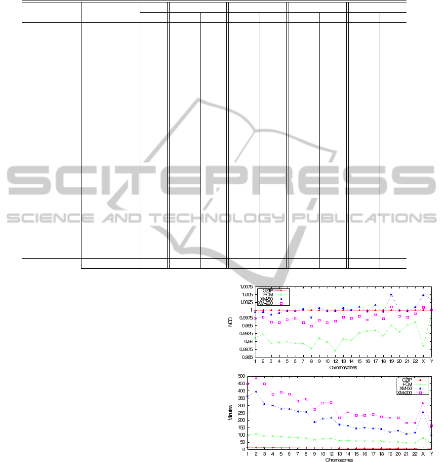
Table 1: The normalized compression distance (NCD) and the time (in minutes) required to compute it using different methods

on the concatenated sequences A and B. The bold values represent the best NCD values.

Sequence A Sequence B Size GZIP XM–50 XM–200 FCM

(Mb) NCD Time NCD Time NCD Time NCD Time

S. pneumoniae L. lactis 4.4 0.9987 0.2 0.9810 1.0 0.9797 1.0 1.0023 1.1

E. coli S. ﬂexneri 9.3 0.9991 0.4 0.2298 2.7 0.2295 2.7 0.4176 2.2

E. coli S. enterica 9.5 0.9992 0.4 0.7776 2.8 0.7743 2.8 0.9748 2.3

A. thaliana C1 A. thaliana C2 50.0 0.9999 2.3 0.9809 19.6 0.9765 19.6 0.9877 10.9

A. thaliana C3 A. thaliana C4 42.0 0.9998 1.9 0.9763 14.0 0.9720 14.0 0.9837 10.7

S. cerevisiae C1 S. cerevisiae C2 1.0 0.9953 0.1 0.9898 0.1 0.9897 0.1 0.9922 0.3

S. cerevisiae C3 S. cerevisiae C4 1.8 0.9975 0.1 0.9945 0.2 0.9944 0.2 0.9947 0.5

S. cerevisiae C5 S. cerevisiae C6 0.8 0.9932 0.1 0.9861 0.1 0.9860 0.1 0.9884 0.2

S. pombe C1 S. pombe C2 10.1 0.9993 0.5 0.9855 2.5 0.9854 2.5 0.9872 2.4

S. pombe C2 S. pombe C3 7.0 0.9993 0.3 0.9941 1.9 0.9940 3.2 0.9948 1.7

M. musculus C5 P. troglodytes C5 325.8 0.9999 14.6 1.0125 370.8 1.0104 524.3 1.0090 90.4

M. musculus C5 H. sapiens C5 326.0 0.9999 14.6 1.0117 363.8 1.0102 542.3 1.0084 91.2

P. troglodytes C5 H. sapiens C5 354.8 0.9999 16.2 0.2475 401.0 0.1762 568.5 0.4743 100.0

H. sapiens C3 H. sapiens C5 371.1 0.9999 17.4 0.9988 441.1 0.9963 601.5 0.9891 104.9

H. sapiens C12 H. sapiens C9 244.5 0.9999 10.9 0.9995 195.7 0.9962 344.5 0.9905 66.9

H. sapiens C12 H. sapiens CY 152.1 0.9999 6.8 1.0029 104.0 0.9997 216.1 0.9992 41.5

H. sapiens C9 H. sapiens CY 137.9 0.9999 6.2 1.0039 73.6 1.0005 177.1 0.9995 38.1

H. sapiens C11 H. sapiens C12 260.0 0.9999 11.2 0.9997 216.8 0.9965 320.7 0.9871 75.3

H. sapiens CY P. troglodytes C5 200.1 0.9999 9.0 1.0004 152.8 0.9996 228.7 0.9971 55.6

H. sapiens C9 M. musculus C5 263.7 0.9999 10.7 1.0099 231.1 1.0080 268.8 1.0073 73.2

A. thaliana C2 S. cerevisiae C2 20.5 0.9998 0.9 1.0001 5.9 1.0001 167.2 1.0001 5.1

A. thaliana C3 S. pombe C3 25.9 0.9999 1.2 1.0002 7.8 1.0002 16.6 1.0004 6.4

S. cerevisiae C1 S. pombe C1 5.8 0.9993 0.3 0.9999 1.5 0.9999 11.3 1.0001 1.4

A. thaliana C4 S. pneumoniae 20.6 0.9998 1.0 1.0007 7.3 1.0007 10.0 1.0013 5.1

Total ≈ 2755 0.9992 123 0.9235 2507 0.9189 3874 0.9493 758

compression distance (NCD) on DNA sequences, be-

cause, as can be seen, it does not show any discrim-

inant capabilities. On the other hand, XM and FCM

seem to be able to distinguish the sequences.

The XM method seems to behave better than FCM

for small sequences and also for sequences that are

very similar. For example, the NCD of E. coli and

S. enterica has a value very small and we know from

(Zhao et al., 2007) that this has a biological justiﬁ-

cation, since these genomes have a strong structural

relation. However, XM is much more time consum-

ing than FCM to accomplish the task.

The FCM method seems to perform better in

sequences that are somewhat dissimilar and large.

A few examples are the chromosomes from the

genomes: H. sapiens, P. troglodytes and M. muscu-

lus. Moreover, as already mentioned, it is more time

efﬁcient than XM. To verify this observation, we have

ran a complete NCD for every H. sapiens chromo-

some. However, due to space restrictions, in Fig. 1,

we only present the NCD results of chromosome 11

with the rest of the chromosomes (H. sapiens).

In Fig. 1, it is possible to verify that FCM pro-

vides the smallest NCD value and time, comparing

with XM, in all entries. Moreover, FCM reveals some

interesting results that are not unveiled by the other

approaches. This can be observed, e.g., in the relative

Figure 1: Normalized compression distance (NCD) for dif-

ferent methods between the human chromosome 11 and

each of all other human chromosomes (top graph, the NCD

value, bottom graph, the time required).

position of the NCD values regarding the similarity

between chromosome 11 and chromosome X, and be-

tween chromosome 11 and chromosome 12.

We have also studied the inter-chromosomal sim-

ilarities in the H. sapiens genome, has it can be seen

in Fig. 2. There are some aspects that we should point

BIOINFORMATICS 2012 - International Conference on Bioinformatics Models, Methods and Algorithms

310

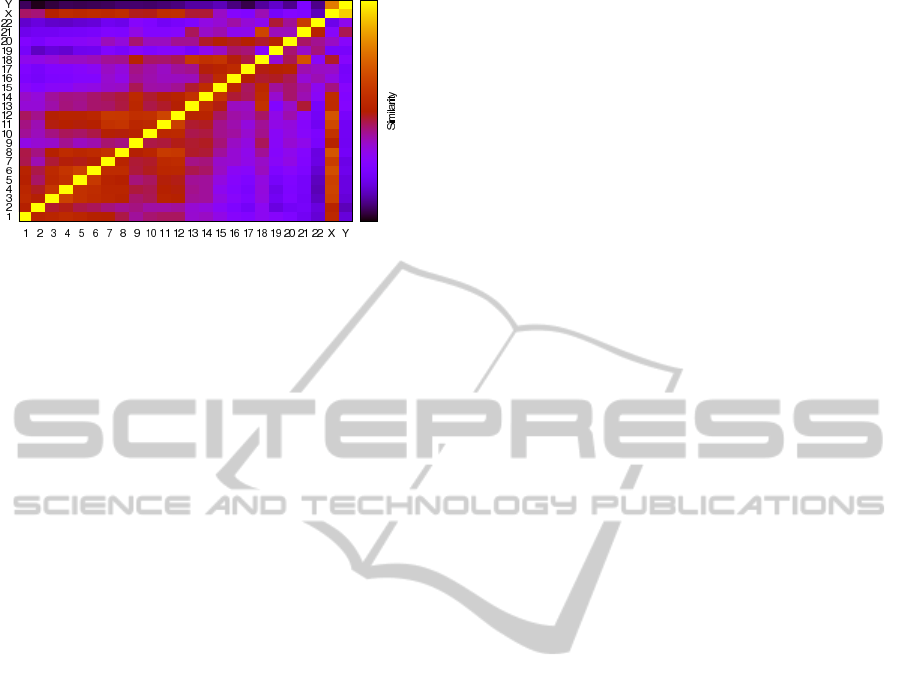
Figure 2: The Human genome inter-chromosomal similar-

ity heat map. On the right side is a bar that indicates the

strength of similarity (highest intensity at the top). The axes

of x and y represent chromosomes.

out: the sexual chromosomes (X-Y) have the larger

similarity among all chromosomes; looking into auto-

somes, the larger similarity is in chromosomes 18/21;

chromosome 12, 18 and X have the overall chromoso-

mal relation; there are relevant similarities is the fol-

lowing pairs: 3/4, 5/6, 11/12, 17/20 and 18/21.

4 CONCLUSIONS

We have developed a method for computing the nor-

malized compression distance based on a mixture

of ﬁnite context models. We have shown that this

method is, on average, better than the state-of-the-

art XM on large and not very similar sequences (the

human genome, for example). Moreover, the time

required to accomplish the task is much lower than

in the XM approach. Using the proposed method,

we have also studied the similarity between chro-

mosomes of the human genome, revealing several

pointed similarities among these chromosomes.

In the future, we intend to create a hybrid solu-

tion using the copy expert and the mixture of ﬁnite-

context models, since these two methods proved to be

of strong functionality and complementarity.

ACKNOWLEDGEMENTS

This work was supported in part by the grant

with the COMPETE reference FCOMP-01-0124-

FEDER-010099 (FCT reference PTDC/EIA-EIA/

103099/2008). Sara P. Garcia acknowledges funding

from the European Social Fund and the Portuguese

Ministry of Education.

REFERENCES

Bennett, C. H., G´acs, P., Vit´anyi, M. L. P. M. B., and Zurek,

W. H. (1998). Information distance. IEEE Trans. on

Information Theory, 44(4):1407–1423.

Cao, M. D., Dix, T. I., Allison, L., and Mears, C. (2007).

A simple statistical algorithm for biological sequence

compression. In Proc. of DCC-2007, pages 43–52,

Snowbird, Utah.

Chaitin, G. J. (1966). On the length of programs for com-

puting ﬁnite binary sequences. Journal of the ACM,

13:547–569.

Cilibrasi, R. and Vit´anyi, P. M. B. (2005). Clustering by

compression. IEEE Trans. on Information Theory,

51(4):1523–1545.

Dix, T. I., Powell, D. R., Allison, L., Bernal, J., Jaeger,

S., and Stern, L. (2007). Comparative analysis of

long DNA sequences by per element information con-

tent using different contexts. BMC Bioinformatics,

8(Suppl. 2):S10.

Gordon, G. (2003). Multi-dimensional linguistic complex-

ity. Journal of Biomolecular Structure & Dynamics,

20(6):747–750.

Kolmogorov, A. N. (1965). Three approaches to the quanti-

tative deﬁnition of information. Problems of Informa-

tion Transmission, 1(1):1–7.

Lempel, A. and Ziv, J. (1976). On the complexity of ﬁ-

nite sequences. IEEE Trans. on Information Theory,

22(1):75–81.

Li, M., Chen, X., Li, X., Ma, B., and Vit´anyi, P. M. B.

(2004). The similarity metric. IEEE Trans. on Infor-

mation Theory, 50(12):3250–3264.

Pinho, A. J., Pratas, D., and Ferreira, P. J. S. G. (2011a).

Bacteria DNA sequence compression using a mixture

of ﬁnite-context models. In Proc. of the IEEE Work-

shop on SSP, Nice.

Pinho, A. J., Pratas, D., Ferreira, P. J. S. G., and Garcia,

S. P. (2011b). Symbolic to numerical conversion of

DNA sequences using ﬁnite-context models. In Proc.

of EUSIPCO-2011, Barcelona.

Pratas, D. and Pinho, A. J. (2011). Compressing the human

genome using exclusively Markov models. In PACBB

2011, vol 93, pages 213–220.

Solomonoff, R. J. (1964). A formal theory of inductive in-

ference. Part I and II. Information and Control, 7(1

and 2):1–22 and 224–254.

Zhao, G., Perepelov, A. V., Senchenkova, et al. (2007).

Structural relation of the antigenic polysaccharides of

E. coli o40, S. dysenteriae type 9, and E. coli k47.

Carbohydrate Research, 342(9):1275–1279.

COMPUTATION OF THE NORMALIZED COMPRESSION DISTANCE OF DNA SEQUENCES USING A MIXTURE

OF FINITE-CONTEXT MODELS

311