TWITTER IMPROVES SEASONAL INFLUENZA PREDICTION

Harshavardhan Achrekar

, Avinash Gandhe

, Ross Lazarus

, Ssu-Hsin Yu

and Benyuan Liu

Department of Computer Science, University of Massachusetts Lowell, Massachusetts, U.S.A.

Scientiﬁc Systems Company Inc, 500 West Cummings Park, Woburn, Massachusetts, U.S.A.

Department of Population Medicine, Harvard Medical School, Boston, Massachusetts, U.S.A.

Keywords:

Flu trends, Online social networks, Prediction.

Abstract:

Seasonal inﬂuenza epidemics causes severe illnesses and 250,000 to 500,000 deaths worldwide each year.

Other pandemics like the 1918 “Spanish Flu” may change into a devastating one. Reducing the impact of

these threats is of paramount importance for health authorities, and studies have shown that effective inter-

ventions can be taken to contain the epidemics, if early detection can be made. In this paper, we introduce

the Social Network Enabled Flu Trends (SNEFT), a continuous data collection framework which monitors ﬂu

related tweets and track the emergence and spread of an inﬂuenza. We show that text mining signiﬁcantly

enhances the correlation between the Twitter and the Inﬂuenza like Illness (ILI) rates provided by Centers

for Disease Control and Prevention (CDC). For accurate prediction, we implemented an auto-regression with

exogenous input (ARX) model which uses current Twitter data, and CDC ILI rates from previous weeks to

predict current inﬂuenza statistics. Our results show that, while previous ILI data from CDC offer a true (but

delayed) assessment of a ﬂu epidemic, Twitter data provides a real-time assessment of the current epidemic

condition and can be used to compensate for the lack of current ILI data. We observe that the Twitter data is

highly correlated with the ILI rates across different regions within USA and can be used to effectively improve

the accuracy of our prediction. Our age-based ﬂu prediction analysis indicates that for most of the regions,

Twitter data best ﬁt the age groups of 5-24 and 25-49 years, correlating well with the fact that these are likely,

the most active user age groups on Twitter. Therefore, Twitter data can act as supplementary indicator to gauge

inﬂuenza within a population and helps discovering ﬂu trends ahead of CDC.

1 INTRODUCTION

Seasonal inﬂuenza epidemics result in about three to

ﬁve million cases of severe illness and about 250,000

to 500,000 deaths worldwide each year (Jordans,

2009). In 1918, the so-called “Spanish ﬂu” killed an

estimated 20-40 million people worldwide, and since

then, human to human transmission capable inﬂuenza

virus has resurfaced in a variety of particularly viru-

lent forms much like “SARS”, “H1N1” against which

no prior immunity exists resulting in a devastating sit-

uation with million of casaulties. Reducing the im-

pact of seasonal epidemics and pandemics such as the

H1N1 inﬂuenza is of paramount importance for pub-

lic health authorities. Studies haveshown that preven-

tive measures can be taken to contain epidemics, if an

early detection is made or if we have some form of

an early warning system during the germination of an

epidemic (Ferguson et al., 2005; Longini et al., 2005).

Therefore, it is important to be able to track and pre-

dict the emergence and spread of ﬂu in the population.

The Center for Disease Control and Prevention

(CDC) (Centers for Disease Control and Prevention,

2009) monitors inﬂuenza-like illness (ILI) cases by

collecting data from sentinel medical practices, col-

lating reports and publishing them on a weekly basis.

It is highly authoritative in the medical ﬁeld but as di-

agnoses are made and reported by doctors, the system

is almost entirely manual, resulting in a 1-2 weeks

delay between the time a patient is diagnosed and the

moment that data point becomes available in aggre-

gate ILI reports. Public health authorities need to be

forewarned at the earliest to ensure effective preven-

tive intervention, and this leads to the critical require-

ment of more efﬁcient and timely methods of estimat-

ing inﬂuenza incidences.

Several innovative surveillance systems have been

proposed to capture the health seeking behaviour

and transform them into inﬂuenza activity. Some of

them include monitering call volumes to telephone

triage advice lines (Espino et al., 2003), over the

counter drug sales (Magruder, 2003), patients visit

Achrekar H., Gandhe A., Lazarus R., Yu S. and Liu B..

TWITTER IMPROVES SEASONAL INFLUENZA PREDICTION.

DOI: 10.5220/0003780600610070

In Proceedings of the International Conference on Health Informatics (HEALTHINF-2012), pages 61-70

ISBN: 978-989-8425-88-1

 2012 SCITEPRESS (Science and Technology Publications, Lda.)

logs to Physicians for ﬂu shots. Google Flu Trends

uses aggregated historical log on online web search

queries pertaining to inﬂuenza to build a comprehen-

sive model that can estimate nationwide ILI activity.

In this paper, we investigate the use of novel data

source, Twitter, which takes advantage of the timeli-

ness of early detection to provide snapshot of the cur-

rent epidemic condition and make inﬂuenza related

predictions on what may lie ahead, on a daily or even

hourly basis. We sought to develop a model which

estimates the number of physician visits per week re-

lated to ILI as reported by CDC.

Our approach assumes Twitter users within United

States as “sensors” and collective message exchanges

showing ﬂu symptoms like “I have Flu”, “down with

swine ﬂu” as early indicators and robust predictors

of inﬂuenza. We expect these posts on Twitter to

be highly correlated to the number of ILI cases in

the population. We analyze tweets, build prediction

models and discover trends within data to study the

characteristics and dynamics of disease outbreak. We

validite our model by measuring how well it ﬁts the

CDC ILI rates over a course of two years from 2009

to 2011. We are interested in looking at how the sea-

sonal ﬂu spreads within the population across differ-

ent regions of USA and among different age groups.

In this paper, we extend our preliminary analy-

sis (Achrekar et al., 2011), and provide continuous

study of tracking emergence and spread of seasonal

ﬂu in the year 2010-2011. Twitter data which demon-

strated high correlation with CDC ILI rate last year,

was suppressed by spurious messages and so text min-

ing techniques were applied. We show that text min-

ing can signiﬁcantly enhance the correlation between

the Twitter data and the ILI data from CDC, providing

a strong base for accurate prediction of ILI rate.

For prediction, we build an auto-regression with

exogenous input (ARX) model where ILI rate of pre-

vious weeks from CDC forms the autoregressive por-

tion of the model, and the Twitter data serve as exoge-

nous input. Our results show that while previous ILI

data from CDC offer a realistic (but delayed) measure

of a ﬂu epidemic, Twitter data provides a real-time

assessment of the current epidemic condition and can

be used to compensate for the lack of current ILI data.

We observe that the Twitter data are in fact highly cor-

related with the ILI data across the different regions

within United States.

Our age-based ﬂu prediction analysis indicates

that for most of the regions, Twitter data best ﬁt the

age groups of 5-24 and 25-49 years, suggesting that

these are likely the most active age groups using Twit-

ter. Using ﬁne-grained analysis on user demographics

and geographical locations along with its prediction

capabilities will provide public health authorities an

insight into existing seasonal ﬂu activities.

This paper is organized as follows: Section 2 de-

scribes applications that harness the collective intel-

ligence of Online Social Network (OSN) users, to

predict real-world outcomes. In Section 3, we give

a brief introduction to our data collection and mod-

elling methodolgy. In Section 4, we introduce our

data ﬁltering technique for extracting relevant infor-

mation from Twitter dataset. Detailed data analysis

are performed to establish correlation with CDC re-

ports on ILI rates. Then we go one step further and

introduce our inﬂuenza prediction model in Section

5. In Section 6, we perform Region-wise and Age-

based analysis of ﬂu activities in the population based

on the Twitter. Finally we conclude in Section 7 and

acknowledgements are provided in Section 8.

2 RELATED WORK

A number of studies have been conducted on different

forms of social networks like Del.icio.us, Facebook

and Wikipedia etc. Ginsberg et al. approach for es-

timating Flu trends suggests that relative frequency

of certain search terms are good indicators of per-

centage of physician visits in which a patient presents

inﬂuenza-like symptoms (Ginsberg et al., 2009). Cu-

lotta used a document classiﬁcation component to ﬁl-

ter misleading messages out of Twitter and showed

that a small number of ﬂu-related keywords can fore-

cast future inﬂuenza rates (Culotta, 2010).

Twitter has been used for real-time notiﬁca-

tions such as large-scale ﬁre emergencies, earthquake

(Sakaki et al., 2010), downtime on services provided

by content providers (Motoyama et al., 2010) and

live trafﬁc updates. There have been efforts in utiliz-

ing twitter data for measuring public interest/concern

about health-related events (Signorini et al., 2011),

predicting national mood, forecasting box-ofﬁce rev-

enues for movies (Sitaram and Huberman, 2010), in-

formation diffusion in social media (Leskovec et al.,

2009), currency tracing, performing market and risk

analysis (Jansen et al., 2009) and analysing political

tweets to establish the correlations between buzz on

Twitter and election results (Nardelli, 2010) etc.

3 DATA COLLECTION

We describe our data collection methodology by in-

troducing SNEFT architecture, provide description of

our dataset, explore strategies for data cleaning, apply

ﬁltering techniques in order to perform quantitative

HEALTHINF 2012 - International Conference on Health Informatics

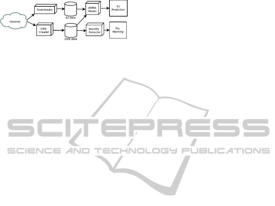
Figure 1: The system architecture of

SNEFT

spatio-temporal analysis.

3.1 SNEFT Architecture

We propose Social Network Enabled Flu Trends

(

SNEFT

) architecture along with its crawler, predic-

tor and detector components, as our solution to pre-

dict ﬂu activity ahead of time with certain accuracy.

CDC ILI reports and other inﬂuenza related data are

downloaded into “ILI Data” database from their cor-

responding websites (e.g., CDC (Centers for Disease

Control and Prevention, 2009)). A list of ﬂu related

keywords (“Flu” , “H1N1” and “Swine Flu”) that are

likely to be of signiﬁcance are used by OSN Crawler

as inputs into public search interfaces to retrieve pub-

licly available posts having mention of those key-

words. Relevant information about the posts are col-

lected along with the relative keyword frequency and

stored in a spatio-temporal “OSN Data” database for

further data analysis.

Autoregressive Moving Average (ARMA) model

is used to predict ILI incidence as a linear function of

current and past OSN data and past ILI data thus pro-

viding a valuable “preview” of ILI cases well ahead

of CDC reports. Novelty detection techniques can be

used to continuously monitor OSN data, and detect

transition in real time from a “normal” baseline situ-

ation to a pandemic using the volume and content of

OSN data enabling

SNEFT

to provide a timely warn-

ing to public health authorities for further investiga-

tion and response.

3.2 Twitter Crawler

In this section we brieﬂy describe the methodology

for collecting our dataset. Based on the search API

provided by Twitter, we developcrawlers to fetch data

at regular time intervals.

The twitter search service accepts single or mul-

tiple keywords using conjunctions (“ﬂu” OR “h1n1”

OR “#swineﬂu”) to search for relevant tweets. Search

results are typically 15 tweets (maximum 50) per

page up to 1,500 tweets arranged in chronologically

decreasing order, obtained from a real time stream

known as the public timeline. The tweet has the User

Name, the Post with status id and the Timestamp at-

tached with each post. From the twitter username, we

can get the number of followers, number of friends,

his/her proﬁle creation date, location and status up-

date count for every user. The location ﬁeld helps

us in tracking the current/default location of a user.

Geo location codes are present in a location enabled

mobile tweet. For all other purposes, we assume the

location attribute within the proﬁle page to be his/her

current location and pass it as an input to Google’s lo-

cation based web services to fetch geo-location codes

(i.e., latitude and longitude) along with the country,

state, city with a certain accuracy scale. All the data

extracted from posts and proﬁle page are stored in a

spatio-temporal “OSN data” Database.

We apply ﬁlters to get quantitative data within

Unites States and exclude organizations and users

who posts multiple times during the day on ﬂu related

activities. This data is fed into the Analysis Engine

which has a detector and ARMA predictor model.

The visualization tools and reporting services gener-

ate timely visual and data centric reports on the ILI

situation. CDC monitors Inﬂuenza-like illness cases

within USA by collecting data about number of Hos-

pitalizations, percentages weighted ILI visits to physi-

cians etc and publishes it online. We download the

CDC data into “ILI data” database to compare our re-

sults.

4 DATA SET

In this section we brieﬂy describe our datasets used

for inﬂuenza prediction. Since Oct 18, 2009, we have

searched and collected tweets and proﬁle details of

Twitter users who mentioned about ﬂu descriptors in

their tweets. The preliminary analysis for the year

2009-2010 is documented in (Achrekar et al., 2011).

For 2010-2011,so far we have4.5 million tweets from

1.9 million unique users. Twitter allows its users to

set their location details to public or private from the

proﬁle page or mobile client. So far our analysis on

location details of Twitter dataset suggest that 22%

users on Twitter are within USA, 46% users are out-

side USA and 32% users have not published their lo-

cation details.

Initial stage analysis for the period 2009-2010, in-

dicated a strong correlation between CDC and Twit-

ter data on the ﬂu incidences (Achrekar et al., 2011).

However results for the year 2010-2011 showed a sig-

niﬁcant drop in the correlation coefﬁcient from 0.98

to 0.47. In an attempt to investigate such a drastic

drop in correlation we looked at data samples and

found spurious messages which suppressed the actual

data. To list a few, tweets like “I got ﬂu shot today.”,

TWITTER IMPROVES SEASONAL INFLUENZA PREDICTION

“#nowplaying Vado - Slime Flu..i got one recently!”

(slime ﬂu is the name of a debut mixtape from an

artist V.A.D.O. released in 2010) are false alarms of

ﬂu. In the year 2009-2010, swine ﬂu event was so

evident that the noise did not signiﬁcantly affect the

correlation that existed then. To mitigate this prob-

lem, we removed the spurious tweets using a ﬁlter-

ing technique that trains a document classiﬁer to label

whether a message is indicative of ﬂu event or not.

4.1 Text Classiﬁcation

In an information retrieval scenario, text mining seeks

to extract useful information from unstructured tex-

tual data. Using simple “bag-of-words” text repre-

sentations technique based on vector space, our algo-

rithm classiﬁes tweets wherein user mentions about

having acquired ﬂu himself or having observered ﬂu

among his friends, family, relatives, etc. Accuracy

of such a model is highly dependent on how well

trained our model is, in terms of precision, recall and

F-measure.

The set of possible labels for a given instance can

be divided into two subsets, one of which are consid-

ered “relevant”. To create such an annotated dataset

which demands human intelligence, we use Amazon

Mechanical Turks to manually classify a sample of

25,000 tweets. Every tweet is classiﬁed by exactly

three Turks and the majority classiﬁed result is at-

tached as the ﬁnal class for that tweet.

The training dataset is fed as an input to different

classiﬁers namely decision tree (J48), Support Vec-

tor Machines (SVM) and Naive Bayesian. For ef-

ﬁcient learning, some conﬁgurations that we did in-

corporate within our text classiﬁcation algorithm in-

cludes setting term frequency and inverse document

frequency(tf-idf) weighting scheme, stemming, using

stopwords list, limiting number of words to keep (fea-

ture vector set) and reordering class. Based on the re-

sults shown in Table 1, we conclude that SVM classi-

ﬁer with highest precision and recall rate outperforms

other classiﬁers when it comes to text classiﬁcation

for our data set. Application of SVM on unclassiﬁed

data originating from within USA resulted in Twitter

dataset with 280K positively classiﬁed tweets from

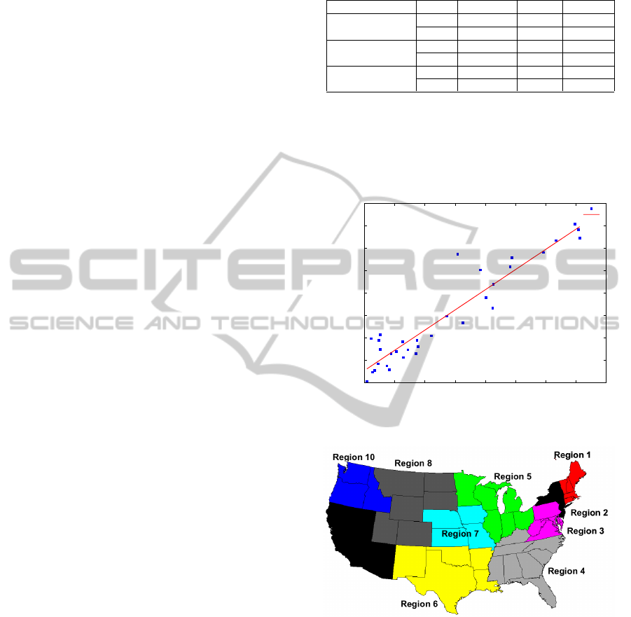
187K unique twitter users. In order to gauge if the

number of unique twitter users mentioning about ﬂu

per week is a good measure of the CDC’s ILI re-

ported data, we plot (in Figure 2) the number of twit-

ter users/week against the percentage of weighted ILI

visits, which yields a high Pearson correlation coefﬁ-

cient of 0.8907.

Thus increase in the users tweeting about ﬂu is ac-

companied by increase in percentage of weighted ILI

Table 1: Text Classiﬁcation 10 fold cross validation results.

Classiﬁer Class Precision Recall F-value

J48

Yes 0.801 0.791 0.796

No 0.813 0.704 0.755

Naive Bayesian

Yes 0.725 0.829 0.773

No 0.813 0.704 0.755

SVM

Yes 0.807 0.822 0.814

No 0.829 0.814 0.822

visits reported by CDC in the same week. However

the marked outlier present in Twitter data as identi-

ﬁed in Figure 2 is coherent with Google Flu Trends

data when high tweet volume were witnessed in the

week starting January 2, 2011.

4000

5000

6000

7000

8000

9000

10000

11000

12000

1 1.5 2 2.5 3 3.5 4 4.5 5

Number of Twitter users posting per week

% ILI visit

Outlier

% ILI visit v/s Twitter users

Fitted line

Figure 2: Number of Twitter users per week versus percent-

age of weighted ILI visit by CDC.

Figure 3: Regionwise Division of USA into ten Regions.

CDC has divided USA into 10 regions as shown

in Figure 3. CDC publishes their weekly reports on

percentage weighted ILI visits collated from its ten

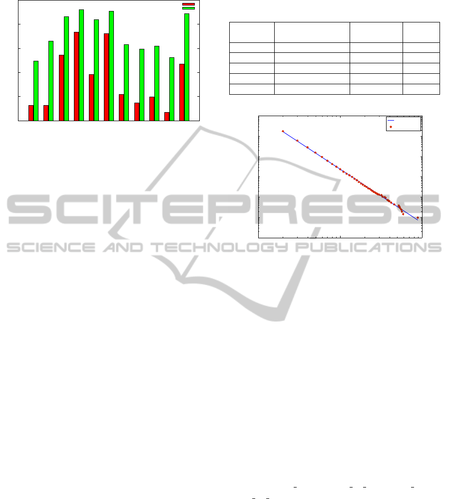
regions and aggregates for USA. Figure 4 compares

the Twitter dataset with CDC reports with and with-

out text classiﬁcation for each of the ten regions de-

ﬁned by CDC and USA as a whole. We observe

that the correlation coefﬁcients have signiﬁcantly im-

proved with text classiﬁcation, across all the regions

and USA overall. Thus our text classiﬁcation tech-

niques plays a vital role in improving the overall de-

tection and prediction performance.

HEALTHINF 2012 - International Conference on Health Informatics

0.2

0.4

0.6

0.8

Region 1

Region 2

Region 3

Region 4

Region 5

Region 6

Region 7

Region 8

Region 9

Region10

USA

Correlation Coefficient

CDC defined Regions and overall USA

Without Text Classification

With Text Classification

Figure 4: Classiﬁed Twitter dataset achieves higher correla-

tion with CDC reports on Nationwide and Regional levels.

4.2 Data Cleaning

The Twitter dataset required data cleaning to discount

retweets and successive posts from same users within

syndrome elapsed time.

• Retweets: A retweet is a post originally made by

one user that is forwarded by another user. For

ﬂu tracking, a retweet does not indicate a new ILI

case, and thus should not be counted in the analy-

sis. Out of 4.5 million tweets we collected, there

are 541K retweets, accounting for 12% of the total

number of tweets.

• Syndrome elapsed time: An individual patient

may have multiple encounters associated with a

single episode of illness (e.g., initial consultation,

consultation 1–2 days later for laboratory results,

and follow-up consultation a few weeks later). To

avoid double counting from common pattern of

ambulatory care, the ﬁrst encounter for each pa-

tient within any single syndrome group is reported

to CDC, but subsequent encounters with the same

syndrome are not reported as new episodes until

more than six weeks have elapsed since the most

recent encounter in the same syndrome (Lazarus

et al., 2002). We call this Syndrome Elapse time.

Hence, we created different datasets namely: Twit-

ter dataset with No Retweets (Tweets starting with

RT) and Twitter dataset without Retweets and with

no tweets from same user within certain syndrome

elapsed time.

When we compared different datasets mentioned

in Table 2 with CDC data, we found that Twitter

dataset without Retweets showed a high correlation

(0.8907) with CDC Data. As opposed to a common

practice in public health safety, where medical exam-

iners within U.S. observe a syndrome elapse time pe-

riod of six weeks, user behaviour on Twitter follows a

Table 2: Correlation between Twitter Dataset and CDC

along with its Root Mean Square Errors(RMSE).

Retweets Syndrome Elapse Correlation RMSE

Time coefﬁcient errors

No 0 week 0.8907 0.3796

No 1 week 0.8895 0.3818

No 2 week 0.8886 0.3834

No 3 week 0.886 0.3878

No 4 week 0.8814 0.3955

−6

−5

−4

−3

−2

−1

Number of Tweets x

Pr(X>=x)

Fitted Line

CCDF

Figure 5: Complementary Cumulative Distribution function

(CCDF) of the number of tweets by same users.

trend wherein we do not ignore successive posts from

same user. Thus Twitter dataset without Retweets is

our choice of dataset for all subsequent experiments.

From Figure 5, we observe that Complemen-

tary Cumulative Distribution function (CCDF) of the

number of tweets posted by same individual can be

ﬁtted by a power law function of exponent -2.6429

and coefﬁcient of determination (R-square) 0.9978

with a RMSE of 0.1076 using Maximum likelihood

estimation. Most people tweet very few times (e.g.,

82.5% of people only tweet once and only 6% of peo-

ple tweet more than two times).

Most of these high-volume tweets are created

by health related organization, who tweet multi-

ple time during a day and users who subscribe

to ﬂu related RSS feeds published by these orga-

nizations. “Flu alert”,“swine ﬂu pro”, “live h1n1”,

“How To Tips”, “MedicalNews4U” are examples of

such agencies on Twitter.

5 PREDICTION MODEL

The correlation between Twitter activity and CDC re-

ports can change due to a number of factors. Annual

or seasonal changes in ﬂu-related trends, for instance

vaccination rates that are affected by health cares, re-

sult in the need to constantly update parameters relat-

TWITTER IMPROVES SEASONAL INFLUENZA PREDICTION

ing Twitter activity and ﬂu activity. However, partic-

ularly at the beginning of the inﬂuenza season, when

prediction is of most signiﬁcance, enough data may

not be available to accurately perform these updates.

Additionally predicting changes in ILI rates simply

due to changes in ﬂu-related Twitter activity can be

risky due to transient changes, such as changes in

Twitter activity due to ﬂu-related news.

In order to establish baseline for the ILI activity

and to smooth out any undesired transients, we pro-

pose the use of Logistic Autoregression with exoge-

nous inputs (ARX). Effectively, we attempt to predict

a CDC ILI statistic during a certain week by using

Twitter activity and CDC data from previous weeks.

The prediction of current ILI activity using ILI ac-

tivity from previous weeks forms the autoregressive

portion of the model, while the Twitter data from pre-

vious weeks serve as exogenousinputs. By CDC data,

we refer to the percentage of visits to a physician for

ILI (also called as ILI rate).

5.1 Inﬂuenza Model Structure

Although the percentage of physician visits is be-

tween 0% and 100%, the number of Twitter users is

bounded below by 0. Simple Linear ARX neglects

this fact in the model structure. Therefore, we intro-

duce a logit link function for CDC data and a loga-

rithmic transformation of the Twitter data as follows:

Logistic ARX Model.

log



y(t)

1− y(t)



∑

i=1

log



y(t −i)

1− y(t − i)



n−1

∑

j=0

log(u(t − j)) + c+ e(t)

(1)

where t indexes weeks, y(t) denotes the percentage of

physician visits due to ILI in week t, u(t) represents

the number of unique Twitter users with ﬂu related

tweets in week t, and e(t) is a sequence of indepen-

dent random variables. c is a constant term to account

for offset. In our tests, the number of unique Twitter

users u(t) is deﬁned as Twitter users without retweets

and having no tweets from the same user within syn-

drome elapsed time of 0 week. The ﬂu related tweets

are deﬁned as tweets with keywords “ﬂu”, “H1N1”

and “swine ﬂu”. The rationale for the model struc-

ture in Eq. (1) is that Twitter data provides real-time

assessment of ﬂu epidemic. However, the Twitter

data may be disturbed at times by events related to

ﬂu, such as news reports of ﬂu in other parts of the

world, but not necessarily to local people actually get-

ting sick due to ILI. On the other hand, the CDC data

provides a true, albeit delayed, assessment of a ﬂu epi-

demic. Hence, by using the CDC data along with the

Twitter data, we may be able to take advantage of the

timeliness of the Twitter data while overcoming the

disturbance that may be present in the Twitter data.

The objective of the model is to provide timely

updates of the percentage of physician visits. To pre-

dict such percentage in week t, we assume that only

the CDC data with at least 2 weeks of lag is avail-

able for the prediction, if past CDC data is present in

a model. The 2-week lag is to simulate the typical de-

lay in CDC data reporting and aggregation. For the

Twitter data, we assume that the most recent data is

always available, if a model includes the Twitter data

terms. In other words, the most current CDC or Twit-

ter data that can be used to predict the percentage of

physician visits in week t is week t-2 for the CDC data

and week t for the Twitter data.

In order to predict ILI rates in a particular week

given current Twitter data and the most recent ILI data

from the CDC we must estimates the coefﬁcients, a

and c in Eq. (1). Also, in practice, the model orders

m and n are unknown and must be estimated. In our

experiment, we vary m from 0 to 2 and n from 0 to 3

in Eq. (1) in order to obtain the best values of m and

n to use for prediction. Intuitively, this answers the

question of how many weeks of Twitter and ILI data

should be used to predict the ILI activity in the cur-

rent week. Within the ranges examined, m = 0 or n =

0 represent models where there are no CDC data, y, or

Twitter data, u, terms present. Also, if m = 0 and n = 1,

we have a linear regression between Twitter data and

CDC data. If n = 0, we have standard auto-regressive

(AR) models. Since the AR models utilize past CDC

data, they serve as baselines to validate whether Twit-

ter data provides additional predictive power beyond

historical CDC data.

Prediction with Logistic ARX Model. To predict

the ﬂu cases in week t using the Logistic ARX model

in Eq. (1) based on the CDC data with 2 weeks of

delay and/or the up-to-date Twitter data, we apply the

following relationship:

log



ˆy(t)

1− ˆy(t)



= a

log



ˆy(t − 1)

1− ˆy(t − 1)



∑

i=2

log



y(t −i)

1− y(t − i)



n−1

∑

j=0

log(u(t − j)) (2)

log



ˆy(t − 1)

1− ˆy(t − 1)



∑

i=1

log



y(t −i− 1)

1− y(t − i− 1)



n−1

∑

j=0

log(u(t − j− 1)) (3)

where ˆy(t) represents predicted CDC data in week t.

HEALTHINF 2012 - International Conference on Health Informatics

It can be veriﬁed from the above equations that to pre-

dict the CDC data in week t, the most recent CDC

data is from week t − 2. If the CDC data lag is more

or less than two weeks, the above equations can be

easily adjusted accordingly.

5.2 Cross Validation Test Description

Based on ARX model structure in Eq. (1), we con-

ducted tests using different combinations of m and

n values. We currently have 33 weeks with both

Twitter activity and CDC data available (10/3/2010–

05/15/2011). Due to limited data samples, we adopted

the K-fold cross validation approach to test the predic-

tion performance of the models.

In a typical K-fold cross validation scheme, the

dataset is divided into K (approximately) equally

sized subsets. At each step in the scheme, one such

subset is used as the test set while all other subsets

are used as training samples in order to estimate the

model coefﬁcients. Therefore, in a simple case of a

30-sample dataset, 10-fold cross-validation would in-

volve testing 3-samples in each step, while using the

other 27 samples to estimate the model parameters.

In our case, the cross-validation scheme is some-

what complicated by the dependency of the sample

y(t) on the previous samples, y(t − 1), . . . , y(t − m)

and u(t), . . . , u(t− n+ 1) (see Eq. (1) ). Therefore, the

ﬁrst sample that can be predicted is y(max(m+ 1, n))

not y(1). In fact, since we are predicting “two weeks

ahead” of the available CDC data, the ﬁrst sample

that can be estimated is actually y(max(m + 2, n +

1)). Since, prediction equations cannot be formed

for y(1), . . . , y(max(m+ 2, n+ 1) − 1), those samples

were not considered in any of the K subsets during

our experiment to be evaluated for prediction perfor-

mance. However, they were still used in the training

set to estimate the values of the coefﬁcients a

and b

in Eq. (1).

Considering the above constraints, our K-fold val-

idation testing procedure is as follows:

1. For each (m, n) pair from m = 0, 1, 2 and n =

0, 1, 2, 3, repeat the following:

(a) Identify F, the index of ﬁrst data sample that

can actually be predicted. F = max(m+ 1, n)

(b) Represent the available data indices as t =

1, . . . , T. Then divide the dataset into K approx-

imately equally sized subsets {S

, S

, . . . , S

with each subset comprising members that have

an approximately equal time interval between

them. For example, the ﬁrst set would be S

{y(F), y(F + K), y(F + 2K), . . . }, the second

would be S

= {y(F + 1), y(F + K + 1), y(F +

2K + 1), . . .} and so on.

Table 3: Root mean squared errors from 10-fold cross vali-

dation. m and n are deﬁned in Eq. (1). The m and n values

in the table specify the model that results in the RMSE in

the corresponding row and column respectively. The lowest

RMSE in the table is highlighed.

n = 0 n = 1 n = 2 n = 3

m = 0 0.5355 0.4814 0.4813

m = 1 0.6331 0.4107 0.4147 0.4314

m = 2 0.5395 0.3957 0.3986 0.4256

, k = 1, . . . , K, obtain the values

of the model parameters a

and b

using all

the other subsets with the least squares estima-

tion technique. Based on the estimated model

parameter values and the associated prediction

equations in Eq. (2), predict the value of each

member of S

2. For each (m, n) pair, we have obtained a pre-

diction of the CDC time-series, y(t) for t =

, . . . , T. Note that F still represents the ﬁrst

time index that can be predicted. However, we

use the subscript mn to emphasize the fact that F

varies depending on the values of m and n. By

comparing the prediction with the true CDC data,

we calculate the root mean-squared error (RMSE)

as follows:

ε =

T − F

max

+ 1

∑

(y(t) − ˆy(t))

(4)

The RMSE is computed over t = F

max

, . . . , T, re-

gardless of techniques and model orders to ensure

fairness in comparison.

5.3 Cross Validation Results

According to the 10-fold cross validation results in

Table 3, the model corresponding to m = 2 and n =

1 has the lowest RMSE. This indicates that current

Twitter data and two most recent ILI data points are

most useful in accurate prediction of inﬂuenza rates.

In general, the addition of Twitter data improves the

prediction with past CDC data alone. For the 10-fold

cross validation results presented in Table 3, for ex-

ample, the AR model (m = 1, n = 0) comprising of

the y(t − 2) term and the constant term for the pre-

diction of y(t) has a RMSE of 0.6331. For the same

m = 1, the model with additional Twitter data u(t)

(i.e. n = 1) has a lower RMSE of 0.4107. We also

observe that using Twitter data (m = 0) alone is in-

sufﬁcient for prediction and that the past ILI rates are

critical in predicting future values, as is evident from

our results. The addition of Twitter data improves the

prediction with past CDC data alone. Therefore, the

TWITTER IMPROVES SEASONAL INFLUENZA PREDICTION

Twitter data provides a real-time assessment of the ﬂu

epidemic (i.e. the availability of Twitter data in week

t in the prediction of physician visits also in week t

as shown in Eq. (2)), while the past CDC data pro-

vides the recent ILI rates in the prediction model. As

shown earlier in the paper, there is strong correlation

between the Twitter data and the CDC data. Hence,

the more timely Twitter data can compensate for the

lack of current CDC data and help capture the cur-

rent ﬂu trend. Finally in Figure 6, we provide a sin-

1.5

2.5

3.5

4.5

w40

w41

w42

w43

w44

w45

w46

w47

w48

w49

w50

w51

w52

w10

w11

w12

w13

w14

w15

w16

w17

w18

w19

w20

percentage of ILI visits

% physician visits (CDC)

Twitter Data

predicted % physician visits

Figure 6: Weekly plot of percentage weighted ILI visits,

positively classiﬁed Twitter dataset and predicted ILI rate

using CDC and Twitter

gle plot for percentage weighted ILI visits, positively

classiﬁed Twitter users and predicted ILI rate using

CDC and Twitter for the year 2010-2011. Note that

the original Twitter data alone would predict higher

ILI rates for the begining and ending parts of the ﬂu

season. Using previous ILI data from CDC offers a

better assessment for making ﬂu predictions.

6 FLU PREDICTION WITHIN

REGIONS AND AGE GROUPS

In this section we discuss the use of Twitter for ﬂu pre-

dictions in speciﬁc population groups. Given the data

available, we are able to study the prediction perfor-

mance in speciﬁc regions of the United States. Also,

with ILI rates provided in different age groups we are

able to study the effectiveness of using Twitter data to

predict ﬂu trends in these age groups. The advantages

of studying performance in subgroups are twofold:

• The differences in Twitter usage among differ-

ent population groups and similar differences in

response amongst people in different population

groups to ILI-like symptoms can result in very

different model parameters and prediction per-

formance when attempting to predict ﬂu activity

among different sections of the population. It is

therefore important to adapt the prediction mod-

els for different population groups.

• In our previous study, it has been shown that there

exists signiﬁcant correlation between Twitter re-

ports and the percentage of ILI cases reported by

CDC. However, much of our analysis is based on

a limited number of data points (31 overlapping

weeks for Twitter and CDC reports for the year

2009-2010 and 33 overlapping weeks for Twitter

and CDC reports for the year 2010-2011) avail-

able during our period of performance evaluation,

with Twitter and ILI data aggregated across the

entire United States. In the year 2009-2010, only

11 out of 31 data points occurred during the weeks

where the ILI rates were signiﬁcant (>2%) and

during this interval, the ILI rates and Twitter re-

ports were steadily decreasing. During the period

2010-2011, 15 out of 33 data points occurred dur-

ing the weeks where the ILI rates were signiﬁcant

(>2%) and during this interval, the ILI rates and

Twitter reports were simultaneously increasing till

they reached their peak in mid February 2011 and

then onwards they both started decreasing.

Due to this limited time frame any claim of high cor-

relation between the two data streams (ILI rates and

Twitter reports) may be viewed with skepticism. This

evaluation was performed as an experiment to see

which age groups the Twitter data ﬁt best. The results

are interesting but not conclusive.

6.1 Regional Twitter and ILI Rates

We analyzed the relationship between the Twitter ac-

tivity and ILI rates across all geographic regions de-

ﬁned by the Health and Human Services (HHS) re-

gions. For reference, the regions are shown on the

USA map in Figure 3.

In studying the regional statistics, we would like

to make some comparisons across regions. For in-

stance (i) when the ILI rate peaks later in a particular

region than the rest of country, do the Twitter reports

also peak later, (ii) is there in relationship between the

decay in ILI rates and the decay in Twitter reports.

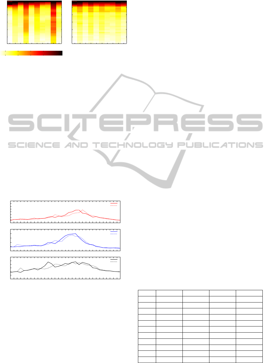
Figure 7 shows, for both ILI and Twitter data, the

relative intensity across the ten Health and Human

Services (HHS) regions (columns) during successive

weeks (rows) in the year 2009-2010. The colormap

used is a scale with white representing low intensity

and black, high intensity. We are comparing ”trends”

among the ILI and Twitter data.

Regional analysis shows that ILI seems to peak

later in the Northeast (Regions 1 and 2) than in the rest

of the country by at least week. The Twitter reports

HEALTHINF 2012 - International Conference on Health Informatics

HHS Region

Week number

1 2 3 4 5 6 7 8 9 10

HHS Region

Week number

1 2 3 4 5 6 7 8 9 10

Figure 7: Heatmap of CDC’s Regionwise ILI data (left) and

Twitter data (right). Colormap scale included (below).

also follow this trend. In Region 9, Region 4 and the

Northeast, the ILI rates seem to drop off fairly slowly

in the weeks immediately following the peaks. This

is also reﬂected in the Twitter reports. Approximately

20-25 weeks after the peak ILI, the northern regions

have lower levels relative to the peaks in the southern

regions. This is also true of the Twitter reports. The

decline in ILI rates is slowest in Region 9.

Figure 8 depicts regionwise ILI prediction perfor-

mance for the year 2010-2011 using our logit model.

We arbitrarily select region 1, region 6 and region 9 to

represent the regions, one each from the East, South

and Western U.S. and plot the true and predicted ILI

values for each of these regions. We observe that

the Twitter reports and ILI rates are in fact correlated

across regions and therefore corroborate our earlier

ﬁndings that Twitter can improve ILI rate prediction.

0.5

1.5

2.5

3.5

w40

w41

w42

w43

w44

w45

w46

w47

w48

w49

w50

w51

w52

w10

w11

w12

w13

w14

w15

w16

w17

w18

w19

w20

Region 1

actual % ILI rate

predicted % ILI rate

w40

w41

w42

w43

w44

w45

w46

w47

w48

w49

w50

w51

w52

w10

w11

w12

w13

w14

w15

w16

w17

w18

w19

w20

% ILI visit

Region 6

actual % ILI rate

predicted % ILI rate

w40

w41

w42

w43

w44

w45

w46

w47

w48

w49

w50

w51

w52

w10

w11

w12

w13

w14

w15

w16

w17

w18

w19

w20

Region 9

actual % ILI rate

predicted % ILI rate

Figure 8: Comparision between Actual and Predicted re-

gional data for Region 1, Region 6 and Region 9.

6.2 Age-based Inﬂuenza Analysis

The differences in Twitter usage and susceptibility to

ﬂu among different demographics can result in very

different prediction model parameters and perfor-

mance when attempting to predict ﬂu activity among

different sections of the population. While any num-

ber of population groups may be deﬁned, the CDC

provides the number of ILI cases by age groups, from

which we can compute the unweighted ILI rates. This

then provides an opportunity to examine the predic-

tion performance amongst different age groups when

predicting ILI using Twitter data. Note that while ILI

rates broken down by age group are available, we do

not have Twitter activity broken down by age group.

Also, it is debatable whether attempting to correlate

Twitter and ILI activity within age groups is of any

value; a signiﬁcant percentage of Twitter activity may

result from family members or friends of the affected

persons. Therefore, we attempt to study the relation-

ship between aggregate Twitter activity over all age

groups with ILI rates in different age groups.

Table 4 shows the Root Relative Squared Error

(RRSE) performance in different age groups for dif-

ferent geographical regions within USA. The RRSE

normalizes the errors to the magnitude of the ground

truth data (in this case the total number of ILI cases

relative to total patients seen by provider) in each age

group. We have highlighted the age groups with the

best match between ILI rates and Twitter data within

each region. In parenthesis, alongside the RRSE val-

ues are the model orders for the autoregressive and x-

components of the general model, (m-n). The ”best”

age-group for prediction in each region is highlighted.

The results indicates that for most of the regions,

Twitter data best ﬁts the age-groups of 5-24 yrs and

25-49 yrs, which correlates well with the fact that

this likely is the most active age groups using Twit-

ter (Twitter, 2011). For Region 6 and 7, the Twitter

activity best ﬁts ILI activity amongst the 0-4 yrs age

group. This is an interesting result which we currently

have no speciﬁc insight into. It should be noted that

for Region 6 and 7, the difference between the ﬁts for

0-4 years and 25-49 years is marginal.

Table 4: Prediction performance (root relative squared er-

ror) using Twitter in different age groups for different geo-

graphical regions within the US. In parenthesis, alongside

the RRSE values are the model orders, (m-n), for the au-

toregressive and x-components of the general model in Eq.

(1) which yield the best performance.

0− 4yrs 5− 24yrs 25− 49yrs 50+ yrs

US 0.5285(0-2) 0.4261(2-2) 0.3577(1-2) 0.4320(1-1)

Reg1 0.5728(2-1) 0.6000(2-2) 0.5499(1-1) 0.7763(1-1)

Reg2 0.6954(0-3) 0.6005(2-1) 0.4965(0-3) 0.5171(1-3)

Reg3 0.4423(0-2) 0.3268(2-2) 0.3066(2-3) 0.3515(1-2)

Reg4 0.5281(0-3) 0.3719(0-1) 0.4792(0-1) 0.5192(0-1)

Reg5 0.6387(1-1) 0.4337(2-3) 0.4300(0-3) 0.5198(1-1)

Reg6 0.3032(0-2) 0.3407(1-2) 0.3564(0-3) 0.4469(0-3)

Reg7 0.5426(2-3) 0.5571(1-3) 0.5492(1-3) 0.6454(2-2)

Reg8 0.6511(1-1) 0.6133(1-2) 0.6649(2-2) 0.6445(2-3)

Reg9 0.7453(2-1) 0.4229(2-1) 0.4690(1-1) 0.6176(2-1)

Reg10 0.8548(2-1) 0.5746(2-1) 0.6462(2-2) 0.7347(2-1)

TWITTER IMPROVES SEASONAL INFLUENZA PREDICTION

The above results show that ﬂu-related Twitter ac-

tivity is more correlated with ﬂu activity with certain

age-groups within the USA population and the cor-

relation may be better in certain regions compared

to others. This does indicate that training prediction

models that are targeted to speciﬁc population seg-

ments is a worthwhile endeavor in a future effort.

7 CONCLUSIONS

In this paper, we have described our approach to

achieve faster, near real time detection and prediction

of the emergence and spread of inﬂuenza epidemic,

through continuoustracking of ﬂu related tweets orig-

inating within United States. We showed that apply-

ing text classiﬁcation on the ﬂu related tweets signif-

icantly enhances the correlation (Pearson correlation

coefﬁcient 0.8907) between the Twitter data and the

ILI rates from CDC.

For prediction, we build an auto-regression with

exogenous input (ARX) model where ILI rate of pre-

vious weeks from CDC formed the autoregressive

portion of the model, and the Twitter data served as

an exogenous input. Our results indicated that while

previous ILI rates from CDC offered a realistic (but

delayed) measure of a ﬂu epidemic, Twitter data pro-

vided a real-time assessment of the current epidemic

condition and can be used to compensate for the lack

of current ILI data.

We observed that the Twitter data was highly cor-

related with the ILI rates across different HHS re-

gions. Our age-based prediction analysis suggested

that for most of the regions, Twitter data best ﬁt the

age groups of 5-24 years and 25-49 years, correlating

well with the fact that these were likely the most ac-

tive age group communities on Twitter. Therefore, ﬂu

trends tracking using Twitter signiﬁcantly enhances

public health preparedness against inﬂuenza epidemic

and other large scale pandemics.

ACKNOWLEDGEMENTS

This research is supported in parts by the National

Institutes of Health under grant 1R43LM010766-01

and National Science Foundation under grant CNS-

0953620.

REFERENCES

Achrekar, H., Gandhe, A., Lazarus, R., Yu, S.-H., and Liu,

B. (2011). Predicting ﬂu trends using twitter data.

IEEE Infocom, 2011 workshop on on Cyber-Physical

Networking Systems (CPNS) 2011.

Centers for Disease Control and Prevention (2009). Flu-

View, a weekly inﬂuenza surveillance report.

Culotta, A. (2010). Detecting inﬂuenza outbreaks by ana-

lyzing twitter messages. Knowledge Discovery and

Data Mining Workshop on Social Media Analytics,

2010.

Espino, J., Hogan, W., and Wagner, M. (2003). Tele-

phone triage: A timely data source for surveillance of

inﬂuenza-like diseases. In AMIA: Annual Symposium

Proceedings.

Ferguson, N. M., Cummings, D. A., Cauchemez, S., Fraser,

C., Riley, S., Meeyai, A., Iamsirithaworn, S., and

Burke, D. S. (2005). Strategies for containing an

emerging inﬂuenza pandemic in southeast asia. Na-

ture, 437:209–214.

Ginsberg, J., Mohebbi, M. H., Patel, R. S., Brammer, L.,

Smolinski, M. S., and Brilliant, L. (2009). Detecting

inﬂuenza epidemics using search engine query data.

Nature, 457:1012–1014.

Jansen, B., Zhang, M., Sobel, K., and Chowdury, A. (2009).

Twitter power:tweets as electronic word of mouth.

Journal of the American Society for Information Sci-

ence and Technology, 60(1532):2169–2188.

Jordans, F. (2009). WHO working on formulas to model

swine ﬂu spread.

Lazarus, R., Kleinman, K., Dashevsky, I., Adams, C.,

Kludt, P., DeMaria, A., Jr., R., and Platt (2002). Use

of automated ambulatory-care encounter records for

detection of acute illness clusters, including potential

bioterrorism events.

Leskovec, J., Backstrom, L., and Kleinberg, J. (2009).

Meme-tracking and the dynamics of the news cy-

cle. International Conference on Knowledge Discov-

ery and Data Mining, Paris, France, 495(978).

Longini, I., Nizam, A., Xu, S., Ungchusak, K., Han-

shaoworakul, W., Cummings, D., and Halloran, M.

(2005). Containing pandemic inﬂuenza at the source.

Science, 309(5737):1083–1087.

Magruder, S. (2003). Evaluation of over-the-counter phar-

maceutical sales as a possible early warning indicator

of human disease. In Johns Hopkins University APL

Technical Digest.

Motoyama, M., Meeder, B., Levchenko, K., Voelker, G. M.,

and Savage, S. (2010). Measuring online service avail-

ability using twitter. Workshop on online social net-

works, Boston, Massachusetts, USA.

Nardelli, A. (2010). Tweetminister.

Sakaki, T., Okazaki, M., and Matsuo, Y. (2010). Earth-

quake shakes twitter users: real-time event detection

by social sensors. In 19th international conference on

World wide web, Raleigh, North Carolina, USA.

Signorini, A., Segre, A. M., and Polgreen, P. M. (2011).

The use of twitter to track levels of disease activity

and public concern in the u.s. during the inﬂuenza a

h1n1 pandemic. PLoS ONE, Volume 6 — Issue 5.

Sitaram, A. and Huberman, B. A. (2010). Predicting the

future with social media. In Social Computing Lab,

HP Labs, Palo Alto, California, USA.

Twitter (2011). Information on twitter users age-wise.

HEALTHINF 2012 - International Conference on Health Informatics