HIERARCHICAL DYNAMIC MODEL FOR

HUMAN DAILY ACTIVITY RECOGNITION

Blanca Florentino-Lia

no, Niamh O’Mahony and Antonio Art

es-Rodr

ıguez

Department of Signal and Communications Theory, Universidad Carlos III de Madrid, Madrid, Spain

Keywords:

Activity recognition, Inertial sensors, Ambulatory monitoring.

Abstract:

This work deals with the task of human daily activity recognition using miniature inertial sensors. The pro-

posed method is based on the development of a hierarchical dynamic model, incorporating both inter-activity

and intra-activity dynamics, thereby exploiting the inherently dynamic nature of the problem to aid the clas-

siﬁcation task. The method uses raw acceleration and angular velocity signals, directly recorded by inertial

sensors, bypassing commonly used feature extraction and selection techniques and, thus, keeping all informa-

tion regarding the dynamics of the signals. Classiﬁcation results show a competitive performance compared

to state-of-the-art methods.

1 INTRODUCTION

The task of human activity recognition using wear-

able inertial sensors is becoming popular in ap-

plications which require context-aware monitoring,

such as ambulatory monitoring of elderly patients

and home-based rehabilitation. In such applica-

tions, knowledge of the activity being carried out by

the patient is vital for providing the context within

which the patient is being monitored and this context-

awareness can help to overcome the limitations asso-

ciated with the use of self reporting in medical assess-

ment. One of the major advantages of such systems is

that they can reduce the frequency of patients’ visits

to medical centers, improving their quality of life and

reducing medical costs.

There are two main methods for human activ-

ity recognition: vision-based, e.g. (Moeslund et al.,

2006), and inertial sensor-based, e.g. (Sabatini et al.,

2005). The main disadvantages of vision-based sys-

tems are that they can only be used in a conﬁned

space, they interfere with the privacy of the individual

and they produce an excessive amount of information

that must be processed. On the other hand, due to re-

cent advances in sensor technologies, inertial sensor

devices have become compact and portable enough

to be unobtrusively attached to the human body. For

this reason, wearable miniature inertial sensors, in-

corporating accelerometers and gyroscopes, have be-

came the ideal platform for human movement moni-

toring (Sabatini et al., 2005), falls detection (Wu and

Xue, 2008), medical diagnosis and treatment (Pow-

ell et al., 2007), and tele-rehabilitation (Winters and

Wang, 2003).

Nowadays, the main challenge in activity recogni-

tion is the development of a system for real-life mon-

itoring applications using wearable sensors. Long

term recording capabilities and unobtrusiveness are

the primary requirements of such systems. The main

constraint for the long term recording capabilities re-

quirement is the battery life of the sensor devices.

This drawback is even more important in real-time

applications, such as fall detection systems. The pro-

cessing of the data in real time can either be done

by the sensor, if it has an on-board processor, or by

transmitting the data wirelessly from the sensor to an

external processor. Both cases result in high battery

consumption and the latter case also requires the pa-

tient to be conﬁned within the range of the wireless

communication system. In order to make the sys-

tem as unobtrusive as possible, the number of sensors

placed on the body should be kept to a the minimum

despite the fact that the larger the number of sensors,

the more activities the system can recognize (Bao and

Intille, 2004). Thus, choosing the number of sensors

is a trade off between performance and usability.

Further to simply identifying which activities a

subject is carrying out, this work proposes to also pro-

vide information regarding of the dynamics of the ac-

tivity itself. There are two beneﬁts to this approach:

(1) the intra-activity dynamics can aid the classiﬁ-

cation task and (2) additional contextual information

Florentino-Liaño B., O’Mahony N. and Artés-Rodríguez A..

HIERARCHICAL DYNAMIC MODEL FOR HUMAN DAILY ACTIVITY RECOGNITION.

DOI: 10.5220/0003781900610068

In Proceedings of the International Conference on Bio-inspired Systems and Signal Processing (BIOSIGNALS-2012), pages 61-68

ISBN: 978-989-8425-89-8

 2012 SCITEPRESS (Science and Technology Publications, Lda.)

could be gained from characteristics of the dynamic

behaviour. With this in mind, we propose a hierar-

chical dynamical model which takes into account two

levels of dynamics: inter-activity and intra-activity.

The model aims to represent the activities as intu-

itively as possible in terms of the patterns present in

the raw data from the sensors. Thus, not only are dif-

ferent activities recognized, but the “events” within a

given activity are also distinguished, for example, the

steps in the case of walking. Three different dynamic

models are described, each one pertaining to a partic-

ular type of activity: the ﬁrst is for stationary activi-

ties like standing, sitting and lying; the second, for ac-

tive movements like walking and running, whilst the

third deals with short-time motions like jumping and

falling.

A further advantage of the proposed system is

that it uses raw signals directly from the sensor, thus

avoiding computationally expensive techniques such

as feature extraction and selection. Because the sys-

tem is designed to capture directly the dynamics of

the signals, activity recognition is achieved with high

accuracy whilst eliminating costly processing tech-

niques.

The paper is organized as follows: in Section 2

the activity recognition literature is reviewed. Section

3 describes the proposed hierarchical dynamic model.

The test procedure is outlined in Section 4, whilst in

Section 5 the results obtained with our model are pre-

sented. Section 6 provides a discussion of the oper-

ation of the proposed method. Finally, in Section 7,

conclusions and future lines of work are discussed.

2 BACKGROUND AND RELATED

WORK

2.1 Sensors and Feature Extraction

The previously published literature in the area of hu-

man activity recognition using inertial sensors is quite

extensive. Most of the published work follows a simi-

lar approach of data collection and processing, as out-

lined in this section.

Perhaps the ﬁrst consideration in any activity

recognition system, is the selection of the type and the

number of sensors, as well as the positions on the hu-

man body where they will be worn. The simplest sen-

sor used in the recent literature is a triaxial accelerom-

eter (Han et al., 2010; Krishnan et al., 2008; He and

Jin, 2008; Khan et al., 2010). In (Frank et al., 2010;

Altun and Barshan, 2010; Zhu and Sheng, 2010), in-

ertial measurement units (IMU), combining triaxial

accelerometers and triaxial gyroscopes, are used to

provide measurements of speciﬁc force and angular

rate, respectively. As has been previously mentioned,

the larger the number of sensors used, the more activi-

ties the system can recognize. Similarly, the choice of

sensor positions on the body is crucial. In the case of

a single sensor, the most popular place is the waist, on

the belt or in the pocket of the trousers (Frank et al.,

2010; Han et al., 2010; He and Jin, 2008). In this

work, a single IMU placed on either the left or right

hip is considered for testing purposes, although the

model is not limited to this conﬁguration.

The ﬁrst processing step is, typically, focused on

the construction of a feature vector derived from the

raw signals of the sensor. In the literature, a large

number of different features have been reported as

being suitable for the classiﬁcation task considered in

this work; (Preece et al., 2009) provides a comparison

of the most popular features. A common approach

is to extract many features (for example in (Krishnan

et al., 2008) thirty-nine features are extracted); then,

dimensionality reduction techniques such as Principal

Component Analysis (PCA) or Linear Discriminant

Analysis (LDA) are used to reduce the size of the fea-

ture vector before classiﬁcation.

In addition to the processing required for feature

extraction and selection, another disadvantage of this

approach is that a predeﬁned window length must be

determined to compute the features. Furthermore, an

overlap is often used between consecutive windows.

The selection of such parameters is somewhat arbi-

trary and there is a lack of agreement on the best

choice; in the literature, the window length varies

widely (e.g. from 16 msec (Han et al., 2010) to 6 sec

(Bao and Intille, 2004)), whilst a 50% overlap is com-

mon.

Once the feature vector has been computed from

the windowed signals, the next step is the develop-

ment of a model that is able to discriminate among

activities. The most popular methods that have been

used to solve this sequential supervised learning prob-

lem are batch supervised learning algorithms and Dy-

namic Bayesian Networks (DBN).

In (Altun and Barshan, 2010), a comparison of

classiﬁcation results using various batch supervised

learning algorithms, including Bayesian Decision

Making (DBM), Least-Squares Method (LSM), k-

Nearest Neighbor (k-NN), Support Vector Machines

(SVM) and Artiﬁcial Neural Networks (ANN) can be

found. Batch supervised learning algorithms, which

ignore the dynamics of the signals, are not consid-

ered in this work. One reason for this is to bypass

the feature extraction step and, furthermore, it will be

seen that consideration the dynamics of the signals

BIOSIGNALS 2012 - International Conference on Bio-inspired Systems and Signal Processing

can give useful information about the type of activity

that is being performed.

In the case of DBN, Hidden Markov Models

(HMM) are the most frequently used. The model pro-

posed in this work is based on HMMs and, so, the

next section will describe, brieﬂy, the theory govern-

ing HMMs and discuss, in detail, their use in the task

of daily human activity recognition.

2.2 Hidden Markov Models

2.2.1 Background

A HMM (Rabiner, 1990) is a probabilistic model that

represents the joint distribution of the observations

and the unobserved (hidden) variable. In this work

the observations are continuous signals of accelera-

tion and angular velocity. The unobserved variable

must be discrete and its possible values are called

states. The proposed hierarchical model in this work,

deﬁnes two different unobserved variables: the activi-

ties (e.g. walking, running, etc.) and the events within

each activity. This will be explained in more detail in

the Section 3.

A ﬁrst order HMM is characterized by the follow-

ing:

• N, the number of states in the model. The individ-

ual states are denoted as S = {S

, S

, . . . , S

}, and

the state at time t as q

• The state transition probability distribution ma-

trix, A = {a

i j

}. This is an N × N matrix where the

element, a

i j

, is the probability of making a transi-

tion from state S

to state S

i j

= P(q

t+1

= S

). (1)

• The emission distribution vector, B = {b

(O)},

where, for state j:

(O) =

∑

m=1

N(O, µ

, U

), (2)

where O is the vector to be modeled, M is the

number of mixtures, c

is the mixture coefﬁcient

for the mth mixture in state j and N is any log-

concave or elliptically symetric density (in our

case we have selected a Gaussian density) with

mean vector µ

and covariance matrix U

for

the mth mixture component in state j.

• The initial state distribution π = {π

} where

= P(q

= S

) (3)

Thus, the HMM is deﬁned by λ = (A, B, π).

For HMMs, the problem of learning the model

parameters is solved by the Baum-Welch algorithm

(Rabiner and Juang, 1993). The Viterbi algorithm

(Viterbi, 1967) is used to compute the most likely se-

quence of states, Q = q

. . . q

, from time t = 0 to

t = T and its probability, given the model and an ob-

servation sequence, O = O

. . . O

2.2.2 HMMs and Activity Recognition

In the literature, there are two main approaches to

solving the activity recognition task using HMMs.

In the ﬁrst approach (Zhu and Sheng, 2010), only

the temporal dependency among activities is modeled

and there is just one HMM, whose number of states

is equal to the number of activities. This model is

very simple and is usually combined with batch su-

pervised learning algorithms. Modeling the temporal

dependencies among the activities allows the system

to model human behavior by forbidding impossible

transitions like, for example, a direct transition from

running to lying down. An example of this approach

can be found in (Zhu and Sheng, 2010) where the

classiﬁcation is done in two steps; ﬁrst, two ANNs are

used for determining whether or not the feature vec-

tor corresponds to a dynamic activity and whether the

movement is vertical or horizontal; then, the fusion of

these two outputs becomes the input to a HMM where

the states are the activities.

In the second approach (Han et al., 2010), one

HMM per activity is modeled. The number of states

of each HMM is a design parameter. The inference

step consists of computing the likelihood of a test se-

quence with each of the HMMs. The activity corre-

sponding to the HMM with the highest likelihood is

the chosen activity. The main drawback of this ap-

proach is that it is necessary to deﬁne a sequence size

in order to learn the models and to infer the test se-

quence. Well-deﬁned sub-units do not exist in the

recorded IMU signals, since human activities are con-

tinuous and any given activity can have a highly vari-

able duration. The sequence size is often selected tak-

ing into account the time interval during which only

one activity exists. In (Han et al., 2010), this is set to

2 seconds. Some disadvantages of this approach are

the requirement to deﬁne the sequence size, that the

temporal dependency among activities is not modeled

and that the HMM of each activity does not represent

the activity itself but a sequence of, for example, 2

seconds of the activity. Thus, dynamic information

is lost by truncating movement patterns and rhythmic

movements.

To overcome this problem, (Oliver et al., 2002)

develop a Layered Hidden Markov Model (LHMM),

in which each layer of the architecture is connected to

the next layer via its inferential results. This represen-

tation segments the problem into distinct layers that

HIERARCHICAL DYNAMIC MODEL FOR HUMAN DAILY ACTIVITY RECOGNITION

operate at different temporal granularities. But, again,

the parameters of the HMMs do not give any intuitive

information about how the person is performing the

activity and it is necessary to arbitrarily deﬁne these

temporal granularities.

As has been shown in this section, there is no con-

sensus on the most discriminative features for use in

an activity recognition system. For this reason, it is

usual to extract a large number of features and, then,

use a dimensionality reduction technique. The ma-

jor drawback of this approach is the computational

cost. Moreover, it has been mentioned that the win-

dow length used to compute the features is another

design parameter that varies widely among previous

studies. With this in mind, this work aims to bypass

the feature extraction step and work directly with the

raw data produced by the sensor.

3 PROPOSED METHOD

The method proposed in this work consists of a hi-

erarchical dynamical model based on HMMs whose

inputs are the raw signals given directly by the sen-

sor. This model takes into account the temporal

dependencies among activities and models each ac-

tivity in terms of acceleration and angular velocity

signals. The hierarchical scheme concept has been

mentioned before in the activity recognition literature

(Khan et al., 2010). In their work, the term hierarchi-

cal is used because the learning process is done in two

steps. First, the type of the activity (static, dynamic

or transition) is recognized, using an ANN, and, then,

the activity itself is determined.

3.1 Hierarchical Dynamical Model

The ﬁnal result of our hierarchical dynamical model

is a single HMM (λ

= (A

, B

, π

)). This ﬁnal

HMM is built up of “sub”-HMMs, one for each ac-

tivity, which are joined to yield the ﬁnal HMM. The

learning process is performed in two stages. In the

ﬁrst stage the intra-activity dynamics are taken into

account, modeling each activity separately with a

unique “sub”-HMM and learning its parameters, as

described in Section 3.1.1. The second stage concate-

nates these HMMs, modeling inter-activity dynamics,

as outlined in Section 3.1.2.

3.1.1 Intra-activity Dynamics

At this level, the hidden variable represents the sig-

niﬁcant events occurring during the activity. These

events are the internal states of the sub-HMMs of each

activity. The individual events, or states, of activity, Z,

are denoted by E

= {E

, ··· , E

} where K

is the

number of states of activity, Z, and the state at time t

is denoted by e

In this ﬁrst stage of the learning process, the joint

probability distribution of the observations, O, and

the events, e, given the activity, Z, (p(e, O|Z)) are

modeled:

p(e, O|Z) =

∏

p(O

, Z)p(e

t−1

, Z). (4)

Each activity can have a different number of events

and a different topology, as detailed in the following.

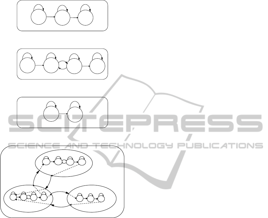
We propose three different topologies, depending

on the type of the activity. All of them have in com-

mon that they have two transient states (the ﬁrst and

the last), that describe the transition from one activity

to another. Each activity must begin in the ﬁrst state,

and once this state is left it cannot be returned to from

within the activity. The only possible transition from

the last state is to itself. This is achieved by forcing

the values of the model parameters to be:

• The transition matrix A

of the activity Z:







0 ··· 0

0 a

··· a

0 0 a

··· a

0 0 0 ··· 1







(5)

• The initial state distribution vector:



1 0 ··· 0



(6)

For stationary activities like standing, sitting and

lying, a left-right model with three states is proposed

(Figure 1). The ﬁrst and the last states are the transient

states and the state in the middle models the perma-

nent state of being seated, for example.

The second model is designed for active move-

ments like walking and running (Figure 2). In this

case there are two intermediate states which represent

the pattern of stepping. These two states are fully

inter-connected in order to model the periodicity of

walking or running.

The last topology models short-time motions like

jumping and falling. This model is made up only of

transient states since there is neither a permanent ac-

tion nor a rhythmic movement (Figure 3).

3.1.2 Inter-activity Dynamics

Once the models of each activity have been deﬁned,

they can be concatenated by means of their transient

states (Figure 4) deﬁning the transition probabilities

BIOSIGNALS 2012 - International Conference on Bio-inspired Systems and Signal Processing

# E

Figure 1: HMM topology for stationary activities.

Figure 2: HMM topology for active movements.

Figure 3: HMM topology for short-time motions.

RUN$

STANDING$

WALK$

Figure 4: Concatenation of the HMMs.

among activities. These transition probabilities model

human behavior; for example, the transition probabil-

ity from walking to standing is higher than the tran-

sition probability from walking to running. Never-

theless, if the activity recognition system is used to

monitor the elderly, the transition probability between

walking and running would be lower than that in the

case of monitoring children.

The result of the concatenation is a single HMM,

= (A

, B

, π

), with twenty-one states, corre-

sponding to all events of all activities as follows:

running (states 1-4), walking (5-8), standing (9-11),

sitting (12-14), lying (15-17), jumping (18-19) and

falling (20-21). The state transition probability ma-

trix of the ﬁnal model, A

, is built up following the

steps below:

(i) Set the transition probability matrixes of the

sub-HMMs in the diagonal transition probabil-

ity matrix of the ﬁnal HMM:







Run

0 0 0 0 0 0

0 A

W lk

0 0 0 0 0

0 0 A

Std

0 0 0 0

0 0 0 A

Sit

0 0 0

0 0 0 0 A

Lie

0 0

0 0 0 0 0 A

Jmp

0 0 0 0 0 0 A

Fll







(7)

(ii) Connect the sub-HMMs. This step is straight-

forward, thanks to the deﬁnition of transient

states, since all the activities must begin at the

ﬁrst state and end at the last state of their sub-

HMM. Thus, we set:

i j

= P(e

t+1

= S

)

= P(act

t+1

= Z

|act

= Z), (8)

for all i 6= j which satisfy the condition that S

is the last state of any activity, Z, and S

is the

ﬁrst state of any other activity, Z

. For exam-

ple, to connect the sub-HMM of running to the

sub-HMM of walking, the value of the param-

eter a

= P(e

t+1

= E

walk

= E

run

) of the ﬁ-

nal HMM will be set to P(act

t+1

= walk|act

run).

(iii) Reset the self-transition probabilities corre-

sponding to the last event of each activity,

i.e. set:

j j

= 1 −

∑

m=1,m6= j

(9)

for each j which satisﬁes the condition, S

∈

run

, E

wlk

, E

Std

, E

Sit

, E

Lie

, E

Jmp

, E

Fll

The emission probabilities of the ﬁnal HMM, B

, are

the corresponding emission probabilities of each sub-

HMM, deﬁned in the ﬁrst stage of the learning pro-

cess.

Finally, the initial state distribution of the ﬁnal

HMM, π

, is deﬁned. In general, the value π

is set

to zero if S

does not correspond to the ﬁrst event of

any sub-HMM. In this work, standing is always con-

sidered as the ﬁrst position.

4 TEST PROCEDURE

4.1 Database Description

In order to facilitate comparison of results with state-

of-the-art results, the database available in (Frank

et al., 2010) has been used for testing the proposed

method. This database consists of 4 hours and 30

HIERARCHICAL DYNAMIC MODEL FOR HUMAN DAILY ACTIVITY RECOGNITION

minutes of activity data from 16 subjects (6 females

and 10 males) aged between 23 and 50 years. Data

were recorded in semi-naturalistic conditions. The

IMU was placed on a belt, either on the right or left

hip, providing 3-axis acceleration and 3-axis angular

velocity signals at a sampling rate of 100 Hz.

The activities labelled in the database are running,

walking, standing, sitting, lying, jumping, falling, as-

cending (from sitting to standing and from lying to

standing), descending, accelerating (from walking to

running) and decelerating (from running to walking).

In the database, there are both training sequences and

benchmark sequences. There are two benchmark se-

quences from two different subjects (Emil and Sinja).

Emil has the IMU placed on his right side and Sinja,

on her left side. These benchmark sequences consist

of a succession of activities. More details of the data

collection and labeling can be found in (Frank et al.,

2010).

4.2 Training

For the purposes of learning the model for each ac-

tivity, sequences corresponding to one single activ-

ity were extracted from the database, to be used as

training data. Therefore, for each activity there are a

different number of sequences with different lengths.

Each HMM learned its parameters using the Baum-

Welsh algorithm. The emission distributions were de-

ﬁned as mixtures of two gaussian distributions with

diagonal covariance matrix.

4.3 Evaluation

The hierarchical dynamic model was tested, using

the benchmark sequences, which were decimated by

a factor of 4. This means that the model can be

used with acceleration and angular velocity signals

recorded at a sampling rate of 25 Hz, allowing the

sensor device to consume less battery. In order to

compute the most likely sequence of events given the

observation sequence, the Viterbi algorithm was used.

Using the knowledge of which set of events corre-

spond to each activity, ﬁnally, the sequence of activi-

ties was obtained.

5 RESULTS

Figure 5 shows the sequence of events for the bench-

mark sequence of Emil. The blue crosses correspond

to the events inferred by the Viterbi algorithm. Events

1 to 4 belong to the activity running, 5 to 8 to the ac-

tivity walking and so on, as listed in Section 3.1.2.

The red circles are the true, labelled activities and

they are aligned in the graph with the last event of

each activity. It should be remembered, here, that

the model proposed in this work does not consider

as activities, the “transition” activities labelled in the

database (i.e. ascending, descending, accelerating and

decelerating), since these events are inherently dealt

with by means of the transient events in the hierar-

chical dynamic model. It can be seen from Figure 5

that the transition activities have, indeed, been incor-

porated by the proposed algorithm into the inferred

intra-activity events. The ﬁgure shows good agree-

ment between true and inferred activities.

0 20 40 60 80 100 120 140 160 180 200

Time (sec)

Events

Emil (f

=25Hz)

RUNNING

WALKING

STANDING

SITTING

LYING

JUMP

FALL

TRANSITIONS

Figure 5: Sequence of events inferred for Emil’s benchmark

sequence.

Tables 1 and 2 show the precision and recall values

of each activity for the benchmark sequences of Emil

and Sinja, respectively. The precision of activity, Z,

is measured as number of samples classiﬁed correctly

as activity, Z, divided by the total number of samples

with inferred label equal to Z. The recall parameter is

the number of samples correctly classiﬁed as activity,

Z, divided by the number of samples whose true label

is Z.

For comparison, Table 3 shows the performance

reported in (Frank et al., 2010), relative to which the

performance of the proposed algorithm is seen to be

competitive.

6 DISCUSSION

The results obtained for Sinja (table 2) are lower than

those for Emil (table 1) because our model does not

deal speciﬁcally with the location of the sensor. The

number of training sequences recorded with the sen-

sor placed on the right side was greater than those

recorded on the left side, so the model has learned,

BIOSIGNALS 2012 - International Conference on Bio-inspired Systems and Signal Processing

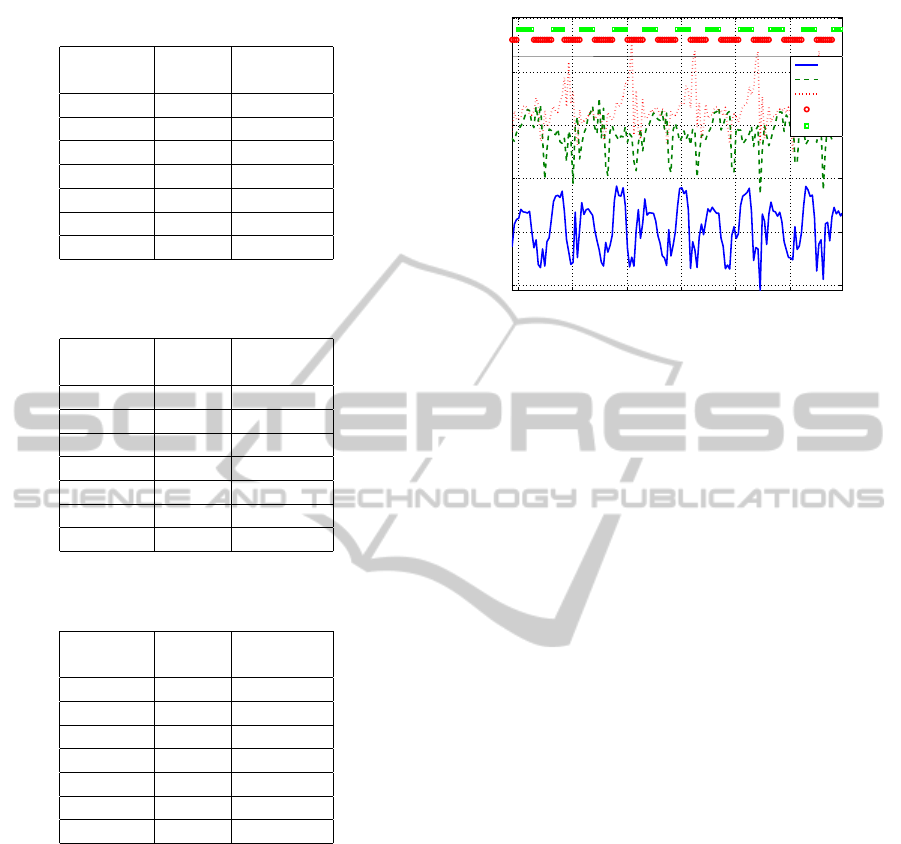
Table 1: Recall and precision for Emil’s benchmark se-

quence (IMU placed on the right side).

Activity Recall Precision

(%) (%)

Running 100 95

Walking 99 97

Standing 96 99

Sitting 100 100

Lying 99 100

Jump 72 96

Fall 100 60

Table 2: Recall and precision for Sinja’s benchmark se-

quence (IMU placed on the left side).

Activity Recall Precision

(%) (%)

Running 100 89

Walking 99 88

Standing 92 100

Sitting 100 100

Lying 100 96

Jump 34 100

Fall 59 82

Table 3: Recall and precision results reported by (Frank

et al., 2010).

Activity Recall Precision

(%) (%)

Running 93 100

Walking 100 98

Standing 98 100

Sitting 100 97

Lying 98 96

Jump 93 93

Fall 100 80

more accurately, the models for a sensor on the right.

In the case of Sinja, the sensor was on the left side.

Nevertheless, the results achieved are considered ac-

ceptable.

This model also gives interesting information in

terms of intra-activity dynamics. Figure 6 shows the

acceleration signals in the x-, y- and z-axes (acc

, acc

and acc

, respectively) and the events inferred during

the activity of walking. The rhythmic transitions be-

tween events, E

W lk

and E

W lk

, are seen to correspond

with the stepping pattern in the acceleration signals.

So, not only has the deﬁnition of the hierarchical dy-

namic model proposed in this work allowed accurate

classiﬁcation of activities without preprocessing of

the raw sensor signals, but the information regarding

the dynamics within the activity itself could also be

used to further characterise the subject’s motion pat-

58 59 60 61 62 63

−15

−10

−5

Time (sec)

m/s

Walking

acc

Wlk

Event sequence

Figure 6: Events inferred for walking and acceleration sig-

nals.

terns and provide useful contextual awareness for the

monitoring system.

Parameterisation of the intra-activity dynamics,

inferred for a particular subject, might have potential

applications in areas such as gait analysis for rehabili-

tation science. However, to be truly useful in this type

of application, it would likely be necessary to improve

the level of detail, by implementing, for example, a

model with a variable number of intermediate states.

7 CONCLUSIONS AND FUTURE

WORK

This work has proposed a new approach to the task

of human daily activity recognition using wearable

inertial sensors. The method presented has two dy-

namic levels, augmenting the information provided

by activity classiﬁcation alone, through the provision

of supplementary information regarding the dynamics

within the activity.

Additionally, our method bypasses the typically

used feature extraction process, which is a computa-

tional bottleneck in current activity recognition meth-

ods. Working directly with the raw signals from the

IMU sampled at a low sampling rate, the inherent dy-

namic nature of human motion is exploited. With this

novel method, results with high precision and recall

rates have been obtained.

Future research plans include developing more so-

phisticated models to take into account variations in

sensor placement as well as implementing the algo-

rithm in real-time. Moreover, a system to extract fea-

tures and parameters from the intra-activity dynam-

ics, provided among the outputs of the new algorithm,

will be developed, to facilitate a detailed analysis of

HIERARCHICAL DYNAMIC MODEL FOR HUMAN DAILY ACTIVITY RECOGNITION

human behaviour in context-aware monitoring sys-

tems.

ACKNOWLEDGEMENTS

This work has been partly supported by Ministe-

rio de Educaci

on of Spain (projects ‘DEIPRO’, id.

TEC2009-14504-C02-01, and ‘COMONSENS’, id.

CSD2008-00010).

REFERENCES

Altun, K. and Barshan, B. (2010). Human activity recog-

nition using inertial/magnetic sensor units. In Pro-

ceedings of the First International Conference on Hu-

man Behavior Understanding, HBU’10, pages 38–51,

Berlin, Heidelberg. Springer-Verlag.

Bao, L. and Intille, S. S. (2004). Activity Recognition from

User-Annotated Acceleration Data. Pervasive Com-

puting, pages 1–17.

Frank, K., Nadales, M. J. V., Robertson, P., and Angermann,

M. (2010). Reliable real-time recognition of motion

related human activities using MEMS inertial sensors.

In ION GNSS 2010.

Han, C. W., Kang, S. J., and Kim, N. S. (2010). Imple-

mentation of HMM-based human activity recognition

using single triaxial accelerometers. IEICE Transac-

tions, 93-A:1379–1383.

He, Z. Y. and Jin, L. W. (2008). Activity recognition from

acceleration data using AR model representation and

SVM. Machine Learning and Cybernetics.

Khan, A. M., Lee, Y.-K., Lee, S. Y., and Kim, T.-

S. (2010). A triaxial accelerometer-based physical-

activity recognition via augmented-signal features and

a hierarchical recognizer. IEEE Transactions on Infor-

mation Technology in Biomedicine, 14:1166–1172.

Krishnan, N. C., Colbry, D., Juillard, C., and Panchanathan,

S. (2008). Real time human activity recognition us-

ing tri-axial accelerometers. In Sensors Signals and

Information Processing Workshop (SENSIP).

Moeslund, T. B., Hilton, A., and Kr

uger, V. (2006). A sur-

vey of advances in vision-based human motion cap-

ture and analysis. Computer Vision and Image Under-

standing, 104:90–126.

Oliver, N., Horvitz, E., and Garg, A. (2002). Layered rep-

resentations for human activity recognition. In Pro-

ceedings of the 4th IEEE International Conference on

Multimodal Interfaces, ICMI ’02, pages 3–, Washing-

ton, DC, USA. IEEE Computer Society.

Powell, H., Hanson, M., and Lach, J. (2007). A wearable

inertial sensing technology for clinical assessment of

tremor. In IEEE Biomedical Circuits and Systems

Conference, BIOCAS 2007., pages 9 –12.

Preece, S. J., Goulermas, J. Y., Kenney, L. P. J., and

Howard, D. (2009). A comparison of feature extrac-

tion methods for the classiﬁcation of dynamic activi-

ties from accelerometer data. IEEE Transactions on

Biomedical Engineering, 56(3):871–879.

Rabiner, L. and Juang, B.-H. (1993). Fundamentals of

Speech Recognition. Prentice Hall, united states ed

edition.

Rabiner, L. R. (1990). Readings in speech recognition. In

Waibel, A. and Lee, K.-F., editors, Readings in speech

recognition, chapter A tutorial on hidden Markov

models and selected applications in speech recogni-

tion, pages 267–296. Morgan Kaufmann Publishers

Inc., San Francisco, CA, USA.

Sabatini, A., Martelloni, C., Scapellato, S., and Cavallo, F.

(2005). Assessment of walking features from foot in-

ertial sensing. IEEE Transactions on Biomedical En-

gineering, 52(3):486 –494.

Viterbi, A. (1967). Error bounds for convolutional codes

and an asymptotically optimum decoding algorithm.

IEEE Transactions on Information Theory, 13(2):260

– 269.

Winters, J. and Wang, Y. (2003). Wearable sensors and tel-

erehabilitation. IEEE Engineering in Medicine and

Biology Magazine, 22(3):56 –65.

Wu, G. and Xue, S. (2008). Portable preimpact fall de-

tector with inertial sensors. IEEE Transactions on

Neural Systems and Rehabilitation Engineering [see

also IEEE Trans. on Rehabilitation Engineering],

16(2):178–183.

Zhu, C. and Sheng, W. (2010). Recognizing human daily

activity using a single inertial sensor. In Proceedings

of the 8th World Congress on Intelligent Control and

Automation (WCICA), pages 282 –287.

BIOSIGNALS 2012 - International Conference on Bio-inspired Systems and Signal Processing