MACHINE LEARNING OF HUMAN SLEEP PATTERNS

BASED ON STAGE BOUT DURATIONS

Francis W. Usher

, Chiying Wang

, Sergio A. Alvarez

2∗

, Carolina Ruiz

and Majaz Moonis

Department of Computer Science, Worcester Polytechnic Institute, Worcester, MA 01609, U.S.A.

Department of Computer Science, Boston College, Chestnut Hill, MA 02467, U.S.A.

Department of Neurology, U. of Massachusetts Medical School, Worcester, MA 01655, U.S.A.

Keywords:

Sleep, Bout duration, Sleep dynamics, Data mining, Clustering, Machine learning.

Abstract:

This paper explores the discovery of patterns in human sleep data based on the duration statistics of continuous

bouts in individual sleep stages during a full night of sleep. Hypnograms from 244 patients are examined.

Stage bout durations are described in terms of the quartiles of their stage bout duration distributions, yielding

15 descriptive variables corresponding to wake after sleep onset, NREM stage 1, NREM stage 2, slow wave

sleep, and REM sleep. Unsupervised Expectation-Maximization clustering is employed to identify distinct

groups of hypnograms based on stage bout durations. Each group is shown to be characterized by bout duration

quartiles of speciﬁc sleep stages, the values of which differ signiﬁcantly from those of other groups (p < 0.05).

Among other sleep-related and health-related variables, several are shown to be signiﬁcantly different among

the bout duration groups found through clustering, while multivariate linear regression fails to yield good

predictive models based on the same bout duration variables used in the clustering analysis. This provides an

example of the successful use of machine learning to uncover naturally occurring dynamical patterns in sleep

data that can also provide sleep-based indicators of health.

1 INTRODUCTION

Sleep is a fascinating process that is not yet fully un-

derstood. Sleep in mammals has been thought to be

controlled by body-wide mechanisms, in order to en-

sure energy conservation and recovery, but it has also

been proposed that sleep may be an emergent prop-

erty of the networks of neurons in the brain (Krueger

et al., 2008). Sleep is known to play a key role in

memory consolidation (Diekelmann and Born, 2010).

The scientiﬁc study of sleep has long used a subdi-

vision of sleep into distinct stages detected through

electroencephalography (EEG), supplemented by the

measurement of other physiological signals (Loomis

et al., 1937) – a technique known as polysomnog-

raphy. A particular stage associated with dream-

ing, the so-called Rapid Eye Movement (REM) stage,

was subsequently identiﬁed (Aserinsky and Kleit-

man, 1953), (Dement and Kleitman, 1957), leading to

currently used staging standards (Rechtschaffen and

Kales, 1968), (Iber et al., 2007) that comprise the light

sleep non-REM (NREM) stages NREM 1 and NREM

∗

Corresponding author.

2, a deep sleep (also known as slow-wave sleep

(SWS)) stage or stages NREM 3/4, as well as REM

sleep. Neuroimaging techniques, including fMRI and

PET, have yielded speciﬁc information about brain

activity in different regions of the brain during each

of these sleep stages (Dang-Vu et al., 2010).

Sleep normally progresses through the various

stages during the course of a full night, albeit in a

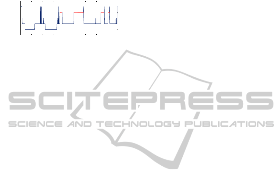
manner that is not predictable in detail. A sample

diagram of the temporal progression of human sleep

stages during the night, known as a hypnogram, is

shown in Fig. 1. This particular diagram was gen-

erated from one of the 244 polysomnographic record-

ings used in the present paper. Some typical features

to note are: most SWS (stages 3 and 4) occurs ear-

lier in the night, a greater amount of REM sleep oc-

curs later in the night, REM and stage 2 alternate

semi-cyclically, and there are brief periods of wake-

fulness throughout the night, after the initial onset of

sleep. Despite some common features across indi-

viduals, the detailed structure of sleep is known to

vary from person to person, and is affected by a va-

riety of factors, from such fundamental physical at-

tributes as body composition (Rao et al., 2009) and

W. Usher F., Wang C., A. Alvarez S., Ruiz C. and Moonis M..

MACHINE LEARNING OF HUMAN SLEEP PATTERNS BASED ON STAGE BOUT DURATIONS.

DOI: 10.5220/0003782500710080

In Proceedings of the International Conference on Health Informatics (HEALTHINF-2012), pages 71-80

ISBN: 978-989-8425-88-1

 2012 SCITEPRESS (Science and Technology Publications, Lda.)

handedness (Propper et al., 2007), to behaviors such

as smoking (Zhang et al., 2006) and the practice of

yoga (Sulekha et al., 2006).

0 100 200 300 400 500 600 700 800 900

SWS

NREM 2

NREM 1

REM

wake

Time (epochs)

Sleep stage

Figure 1: Sample hypnogram from the present study.

Sleep structure is frequently described in terms of

sleep stage composition, that is, in terms of the col-

lection of percentages of time accounted for by var-

ious sleep stages within a night of sleep. For exam-

ple, see (Danker-Hopfe et al., 2005) and (Khasawneh

et al., 2011). While sleep stage composition provides

a good global summary of overall sleep stage content,

it does not capture any information about the dura-

tion and ordering of uninterrupted episodes of differ-

ent sleep stages during the night. Sleep stage dura-

tions havepreviouslybeen used to describe alterations

in sleep dynamics due to health status or ingested

neuroactive substances. For example, in (Bˇrezinov´a,

1976), it is shown that sleep stage durations are af-

fected in speciﬁc ways by age, caffeine, and hypnotic

drug withdrawal. Obstructive Sleep Apnea (OSA) is

shown to alter sleep stage dynamics in (Penzel et al.,

2003) and (Bianchi et al., 2010). Differences in mean

duration of stage 2 bouts between patients with ﬁ-

bromyalgia and normal control subjects have been

described in (Burns et al., 2008). Exponential and

power-law functions have been proposed as models

for the stage duration distributions (Lo et al., 2002),

and the parameter values in these models have been

shown to be affected by health conditions such as

chronic fatigue syndrome (Kishi et al., 2008).

The work reported in the present paper uses a de-

scription of sleep dynamics based on the durations

of continuous, uninterrupted bouts in the different

sleep stages, as well as in wakefulness episodes af-

ter sleep onset. This representation captures tempo-

ral features of sleep that are not considered by stan-

dard sleep composition variables alone. In addition

to the durations of bouts in various sleep stages, it

would be desirable to account for the speciﬁc stage

to which a transition occurs at the end of each stage

bout. However, the information in a full night hypno-

gram appears to be insufﬁcient to adequately model

such stage transitions (Bianchi et al., 2010). In

the present paper, the machine learning technique of

Expectation-Maximization (EM) clustering is used to

group hypnograms into families based on the distri-

butions of their stage bout durations. Hypnograms

within each family are more similar to one another, in

terms of their bout duration statistics, than are hypno-

grams from different families. The prior work (Kha-

sawneh et al., 2011) also uses clustering to study sleep

data, but considers only stage composition, not bout

durations nor other aspects of sleep dynamics. In the

work presented here, each family is shown to be char-

acterized by bout duration statistics for speciﬁc sleep

stages, the values of which are shown to be statisti-

cally signiﬁcantly different from those of other fam-

ilies at the level p < 0.05, even after a suitable cor-

rection has been made for the magniﬁcation of type

I error due to multiple statistical comparisons. Fur-

thermore, several potentially health-related variables

which do not enter into the deﬁnition of the bout du-

ration families, such as a sensation of muscle weak-

ness or paralysis that occurs in emotional situations,

are also shown to differ signiﬁcantly among the bout

duration families identiﬁed through machine learn-

ing, at the level p < 0.05. This is particularly note-

worthy because, in contrast to machine learning, the

widely used statistical technique of multivariate linear

regression does not provide a good predictive model

of this muscle paralysis variable based on the same

bout duration variables. Our results show that ma-

chine learning can uncover interesting dynamical pat-

terns in sleep data, and that such patterns may also be

used to predict selected aspects of individual patient

health based on an all-night sleep study.

2 METHODS

2.1 Human Sleep Data

Fully anonymized human polysomnographic record-

ings were obtained from the Sleep Clinic at Day

Kimball Hospital in Putnam, Connecticut, USA. A

total of 244 recordings were used for the work re-

ported here. Summary statistics for this collection

of sleep data are as in Table 1. The acronyms that

appear in the header row of Table 1 have the fol-

lowing meanings. BMI: Body-Mass Index, the ra-

tio of body weight to height-squared; ESS: Epworth

Sleepiness Scale (Johns, 1991), a measure of day-

time sleepiness based on responses to a questionnaire;

BDI: Beck Depression Inventory(Storch et al., 2004),

a questionnaire-based measure of affective depres-

sion; Mean SaO

: mean level of oxygen-saturated

hemoglobin in the blood.

HEALTHINF 2012 - International Conference on Health Informatics

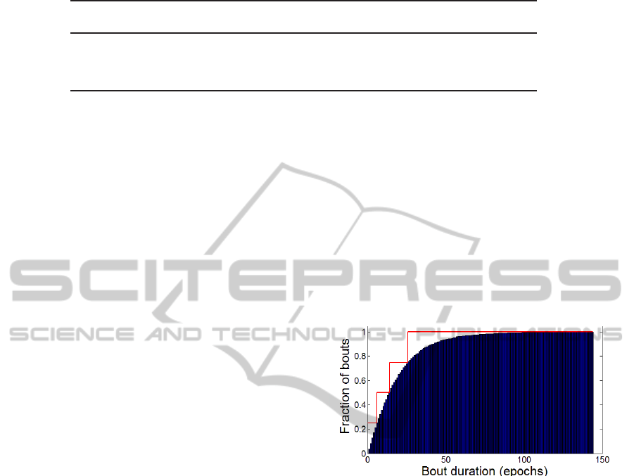
Table 1: Summary statistics of sleep dataset.

Age BMI ESS BDI Mean SaO

Heart rate

(years) (kgm

−2

) (score) (score) (%) (bpm)

Male (n=122) µ± σ 47.4±15.1 33.7±8.1 7.6±5.4 11.5±8.8 93.5±2.9 68.5±11.3

Female (n=122) µ± σ 48.4±14.5 33.7±8.3 7.1±4.8 13.0±7.8 94.6± 1.9 70.8±9.6

Overall (n=244) µ± σ 47.9±14.8 33.7±8.2 7.4±5.1 12.2±8.3 94.1±2.5 69.7±10.5

min–max 20–85 19.2–64.6 0–23 0–48 70.2–97.9 46–99

2.2 Descriptive Data Features

2.2.1 Staging

The polysomnographic recordings were staged in

30-second epochs by expert sleep technicians fol-

lowing the Rechtschaffen and Kales (R & K) stan-

dard (Rechtschaffen and Kales, 1968). R & K NREM

stages 3 and 4 were then combined to obtain a single

slow wave sleep (SWS) stage, resulting in stage labels

that are known (Moser et al., 2009) to provide a good

approximation to the more recently proposed AASM

staging standard (Iber et al., 2007).

2.2.2 Sleep Stage Bouts and Bout Durations

Next, bout durations in epochs were extracted from

each hypnogram. A bout is deﬁned to be a maxi-

mal uninterrupted segment of the given stage within

a given hypnogram. For example, four distinct REM

bouts are visible in Fig. 1. A bout that begins in epoch

t has duration T − t, where T is the ﬁrst epoch after t

such that the sleep stages of the given hypnogram in

epochs t and T are not the same.

2.2.3 Cumulative Distribution Function

The cumulative distribution function (CDF) of the

bout durations was then computed for each sleep

stage. The CDF of stage X is the function F

deﬁned

for each duration, d, as follows (the letter P denotes

probability):

(d) = P(a bout of stage X has duration ≤ d)

With an average of 250 possible bout durations per

stage, this process yields a feature vector of length

approximately 1250 for each data instance.

2.2.4 Bout Duration Quartiles

Selected features of the duration distributions were

used to reduce the dimensionality of the data rep-

resentation. Speciﬁcally, only the three bout dura-

tion quartile values were used to describe each stage,

yielding a 15-dimensional feature vector for each in-

stance. For each stage X, and each index i = 1, 2, 3,

the i-th quartile X.Qi is deﬁned as follows:

X.Qi = argmin

(d) ≥ 0.25i},

where F

is the CDF of stage X. In words, the value

of X.Qi for a given set of hypnograms is the smallest

d for which at least i quarters of the stage X bouts in

the input set have a duration of d or less. As an illus-

tration, the CDF of NREM stage 2 bout durations for

the entire set of 244 hypnograms is shown in Fig. 2,

together with the compressed quartile representation,

visualized as a piecewise constant approximationwith

jumps at the quartile durations.

Figure 2: Stage NREM 2 bout duration CDF with quartiles

visualized as CDF approximation.

2.3 Clustering

2.3.1 Clustering Technique

Unsupervised clustering was applied to the set of 15-

dimensional feature vectors described in section 2.2

to seek objectively deﬁned groups of hypnograms as-

sociated with distinct bout duration distributions. The

technique of Expectation-Maximization (EM) clus-

tering was selected after an experimental comparison

with k-means clustering showed higher stability of the

EM clustering results with respect to pseudorandom

initial parameter variation (see section 3.1). EM per-

forms iterative maximum likelihood estimation of the

cluster parameters (Dempster et al., 1977; Neal and

Hinton, 1998). Clustering experiments were carried

out using the Weka data mining toolkit (Hall et al.,

2009). A mixture of Gaussians is used as the cluster

model, and initial parameter values are found through

k-means clustering.

MACHINE LEARNING OF HUMAN SLEEP PATTERNS BASED ON STAGE BOUT DURATIONS

2.3.2 Measuring Clustering Stability

Stability of clustering results in the presence of pseu-

dorandom parameter initialization was assessed by

comparing the clusters that result from all pairs of 50

seed values for a given value of k. A measure of clus-

tering agreement based on the fraction of pairs of in-

stances that are grouped together in the same cluster

by each of the two clusterings, known as the adjusted

Rand Index (Hubert and Arabie, 1985), was computed

for all pairs of seed values. As compared with the

standard Rand Index (Rand, 1971), the adjusted Rand

Index is much more strict, as it accounts for the de-

gree of matching expected by chance. Subsequent ex-

periments were performed with a clustering of max-

imum mean adjusted Rand Index when compared to

the other 49 tested seed values.

2.4 Statistical Signiﬁcance

Tests of statistical signiﬁcance are employed here to

ensure validity of the ﬁndings at the level p < 0.05,

minimizing the inference of apparent patterns that

may occur due to chance. Speciﬁc statistical hypoth-

esis tests used are described below, together with the

methodology employed to control the type I error rate

due to multiple statistical comparisons.

2.4.1 Multiway and Pairwise Comparisons

When comparing means or medians of several popu-

lations (e.g., clusters), ANOVA or a Kruskal-Wallis

test are used. Likewise, statistical signiﬁcance of

differences of means or medians between pairs of

populations is tested by using either a t-test or

Wilcoxon rank sum test, respectively. ANOVA and

t-tests presuppose normality of the distribution of the

means, a condition that may not hold exactly in all

cases. Nearly all of the comparisons performed in the

present paper involve populations with several dozen

members, and the normality condition is satisﬁed ap-

proximately. In any case, the Kruskal-Wallis and

Wilcoxon rank sum tests do not presuppose normality,

and provide additional conﬁdence regarding statisti-

cal validity. A two-sample Kolmogorov-Smirnov test

is used to compare probabililty distributions without

any assumptions of a particular functional form, and

without targeting any particular statistic such as the

mean or median.

2.4.2 Correction for Increased Type I Error due

to Multiple Comparisons

Several of the results described are obtained through

exploratory data analysis, involving the simultaneous

testing of multiple statistical hypotheses. In any such

situation, the risk of a type I inference error – incor-

rectly rejecting a null hypothesis – increases due to

the accumulation of error over multiple comparisons.

This issue is addressed in the present paper using the

method of (Benjamini and Hochberg, 1995), which

provides rigorous control of the false discovery rate,

that is, of the expected proportion of multiple null hy-

potheses that are incorrectly rejected due to multiple

comparisons. Control of the false discovery rate is

performed at the signiﬁcance level p < 0.05.

3 RESULTS

3.1 Clustering Stability

Table 2 contains the mean observed values of the ad-

justed Rand Index (see subsection 2.3) for EM and k-

means clustering, and k = 2, 3, 4. As shown, the mean

observed value of the adjusted Rand Index for EM is

at least 0.87 for all values of k considered. We note

that the values of the standard Rand Indexfor EM (not

shown) are at least 0.94 over the range k = 2, 3, 4.

The adjusted Rand Index accounts for the degree

of matching expected by chance, and thus produces

more conservative values. The high values obtained

for the adjusted Rand Index show that the EM cluster-

ing obtained is only slightly inﬂuenced by the initial

parameter values, and represents a stable grouping of

the hypnograms. Furthermore, EM consistently out-

performs k-means as regards clustering stability over

the stage bout duration dataset. For this reason, EM

was selected as the clustering algorithm for the work

discussed in the present paper. The seed value 8 was

found to provide an EM clustering of maximum mean

adjusted Rand Index as compared to the other 49 seed

values considered, for each k = 2, 3, 4. All results dis-

cussed subsequently in this paper utilize the EM clus-

tering resulting from the seed value 8.

In passing, we note that variants of the bout du-

ration quartile data representation described in sec-

tion 2.2.4, but using more than 4 quantiles, were also

considered for the present work. The advantage of us-

ing a greater number of quantiles is the ability to de-

scribe ﬁner details in the bout duration distributions.

However, clustering stability was considerably lower

with such representations, and so the decision was

made to use quartiles only.

HEALTHINF 2012 - International Conference on Health Informatics

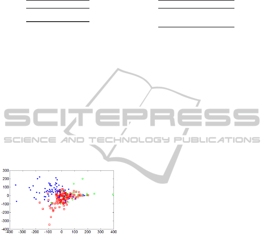
Table 2: Mean adjusted Rand Index stability values.

k 2 3 4

EM 0.99 0.90 0.87

k-means 0.51 0.53 0.36

3.2 Cluster Separation

3.2.1 Visualization of Cluster Separability

The visualization technique of multidimensional scal-

ing (MDS) provides a low-dimensionalnonlinear pro-

jection of a set of dataset in a way that minimizes

distortion of the distances between pairs of data in-

stances (Borg and Groenen, 2005). Fig. 3 shows a

two-dimensional MDS projection of the set of data

instances used in the present paper. The results of

EM clustering did not enter into the generation of the

MDS projection. The EM cluster labels for k = 3 were

used only to determine the glyph (marker) used for

each instance in the visualization shown. The MDS

result shows only moderate separation among the EM

clusters in two dimensions, which indicates that more

than two variables are likely to be needed in order to

achieve high separation. See section 3.2.2.

Figure 3: Multidimensional scaling cluster visualization.

3.2.2 Measurement of Cluster Separation via

Classiﬁcation

Separation among clusters was further assessed quan-

titatively by performing a classiﬁcation task in which

the EM cluster labels are viewed as the target class

attribute, with the variables used for clustering used

as predictive attributes. Classiﬁcation accuracy, the

fraction of instances for which the cluster label is cor-

rectly predicted, and the area under the Receiving Op-

erating Characteristic (ROC) plot (Fawcett, 2003), re-

main consistently above 0.80 in the cases k = 2, 3, 4

for widely used classiﬁcation techniques including

C4.5 (J48) decision tree learning, na¨ıve Bayes, and

multilayer artiﬁcial neural networks (ANN). The area

under the ROC plot accounts for prediction errors on

Table 3: Area Under ROC Graph for Selected Classiﬁers.

classiﬁer k = 2 k = 3 k = 4

ANN 0.94 0.97 0.91

J48 0.88 0.90 0.89

naive Bayes 0.99 0.98 0.98

a per-class basis, and is a better measure of classiﬁ-

cation performance in this context because the class

(cluster) sizes are very dissimilar. Accuracy can

produce overly optimistic results in such situations.

Mean values of the area under the ROC plot for se-

lected classiﬁers appear in Table 3. A 4-fold cross-

validation protocol was employed to control variance

due to data sampling.

Cluster separation is at best moderate in two-

dimensional projections of the bout duration dataset

in terms of the bout duration clustering variables, as

expected based on the MDS visualization in Fig. 3.

An example of moderate cluster separation occurs

with the wake.Q3 and SWS.Q1 bout duration quartile

variables. Use of the rule induction algorithm RIP-

PER (Cohen, 1995) (JRIP) over these predictive vari-

ables alone, with the k = 3 cluster label as the class,

yields, after pruning and simpliﬁcation, the classiﬁca-

tion rules shown in Fig. 4. The ﬁnal rule is a default

rule that is used when the other rules do not apply.

This particular model attains an accuracy of 0.77 and

a mean area under the ROC plot of 0.76. Although the

classiﬁcation performance of the model in Fig. 4 is

unremarkable, it provides an easily understood rough

description of the clusters in the case k = 3. In partic-

ular, it suggests that cluster 2 is associated with high

wake bout durations. More detailed characterizations

of the various clusters are discussed in section 3.3.4.

3.3 Statistical Properties of the Bout

Duration Clusters

3.3.1 Cluster Sizes and Membership

The sizes of the EM bout duration clusters for k =

2, 3, 4 appear in Table 4. There exist relationships

among the three families of clusterings, each of which

corresponds to a value of k in the range 2, 3, 4. These

relationships are observed by examining the detailed

lists of individual instances (not shown) that comprise

the various clusters. A simpliﬁed description of the

relationships among clusterings for different values of

k is the following. Additional characteristics of indi-

vidual clusters are given in Table 5 and discussed in

section 3.3.4.

Relationships between k = 2 and k = 3 Clusters.

The cluster labeled 1 in the k = 2 family splits into

MACHINE LEARNING OF HUMAN SLEEP PATTERNS BASED ON STAGE BOUT DURATIONS

(wake.Q3 >= 50) => cluster=cluster2 (10.0/0.0)

(SWS.Q1 >= 30) => cluster=cluster3 (41.0/2.0)

(SWS.Q1 >= 17) and (6 >= wake.Q3 >= 4) => cluster=cluster3 (13.0/3.0)

=> cluster=cluster1 (180.0/37.0)

Figure 4: JRIP rule model of k = 3 clusters using wake.Q3 and SWS.Q1 only. Coverage/errors in parentheses.

Table 4: Sizes of the bout duration clusters.

k 2 3 4

{211, 33} {148, 19, 77} {127, 15, 48, 54}

the two k = 3 clusters labeled 1 and 3. As discussed

in section 3.3.4 below, the k = 3 cluster 3 portion is

characterized by higher SWS bout duration quartiles

than the k = 3 cluster 1 portion. Two-thirds of the

k = 2 cluster 2 – with higher wakeand lower SWS and

REM bout duration quartiles – retains its identity in

the k = 3 family; the remaining one-third of the k = 2

cluster 2 joins the k = 3 cluster 3. The only inaccuracy

in this description is that 3 of the 33 instances in the

k = 2 cluster 2 join the k = 3 cluster 1.

Relationships between k = 3 and k = 4 Clusters.

In the transition between k = 3 and k = 4, cluster 1

remains largely unchanged (with only 12 of 148 in-

stances leaving cluster 1 and joining cluster 4). Clus-

ter 2 remains mainly within cluster 2 (with 4 of 19

instances joining cluster 4, which has higher mean

REM bout duration quartiles than cluster 2; see sec-

tion 3.3.4). Two-thirds of the k = 3 cluster 3 joins

the k = 4 cluster 2, and the remaining one-third of

k = 3 cluster 3 remains within the k = 4 cluster 3 (8

instances join k = 4 cluster 4). However, the k = 4

cluster 3 retains the characteristic, shared with k = 3

cluster 3, of having the highest SWS bout duration

quartiles among clusters.

3.3.2 Cluster Bout Duration Summary Statistics

The mean, standard deviation, median, and mean ab-

solute deviation of the 15 descriptive variables were

computed for each of the EM clusters, with a view to-

ward establishing statistical differences among clus-

ters. Table 5 provides numerical values of the bout

duration quartile means of the different clusters for

k = 2, 3, 4. Fig. 5, 6, 7 show the mean values of the

15 clustering variables in the cases k = 2, 3, 4, respec-

tively. These ﬁgures suggest that each cluster is char-

acterized by different bout duration quartiles for one

or more of the sleep stages than the other clusters

(e.g., cluster 2 by higher wake duration quartiles).

3.3.3 Multiway Cluster Comparisons

Statistical signiﬁcance of the observed differences in

the means among clusters was assessed by ANOVA

and Kruskal-Wallis tests for multiway comparisons,

and by t, and Wilcoxon rank sum tests for pair-

wise comparisons. A nonparametric two-sample

Kolmogorov-Smirnovtest was also used to determine

differences between pairs of clusters in the overall

distributions of the bout duration quartile variables.

All p-values were corrected for multiple compar-

isons using the Benjamini-Hochberg method on a per

clustering basis, so that reported p-values are upper

bounds on the false discovery rate relative to all ﬁnd-

ings over the given family of k clusters. The results

are as follows. For all clustering families, k = 2, 3, 4,

the wake stage and stage NREM1 duration quartile

variables differ signiﬁcantly among clusters in a mul-

tiway comparison using the Kruskal-Wallis test (p <

0.05). ANOVA results are in agreement with Kruskal-

Wallis, with the exception that the inter-cluster differ-

ence in the quartile variable REM.Q1 is not found to

be signiﬁcant for k = 2, 3. Additionally, both Kruskal-

Wallis and ANOVA ﬁnd highly signiﬁcant (p < 10

−6

)

differences among clusters in the SWS bout duration

quartile variables for k = 3, 4. In contrast, the dif-

ferences in the stage NREM2 bout duration quartiles

among clusters are not found to be signiﬁcant for any

of the clustering families, k = 2, 3, 4. Pairwise statis-

tical comparisons provide additional information, and

are discussed in section 3.3.4 below.

3.3.4 Pairwise Comparisons. Bout Duration

Characteristics of Individual Clusters

The following are a few noteworthy statistically sig-

niﬁcant differences in bout durations. The reader is

also referred to Table 5, and Fig. 5, 6, 7 in conjunction

with this discussion. Below, the precise family (value

of k) is sometimes omitted, in case in which bout du-

ration characteristics of a particular cluster number

are qualitatively similar for different values of k.

Cluster 1. Clusters 1 and 3 share the property that

their median wake bout duration quartiles are sig-

niﬁcantly lower than for clusters 2 and 4 (Wilcoxon

p < 0.05). On the other hand, cluster 1 has signiﬁ-

cantly lower SWS bout duration quartiles than clus-

HEALTHINF 2012 - International Conference on Health Informatics

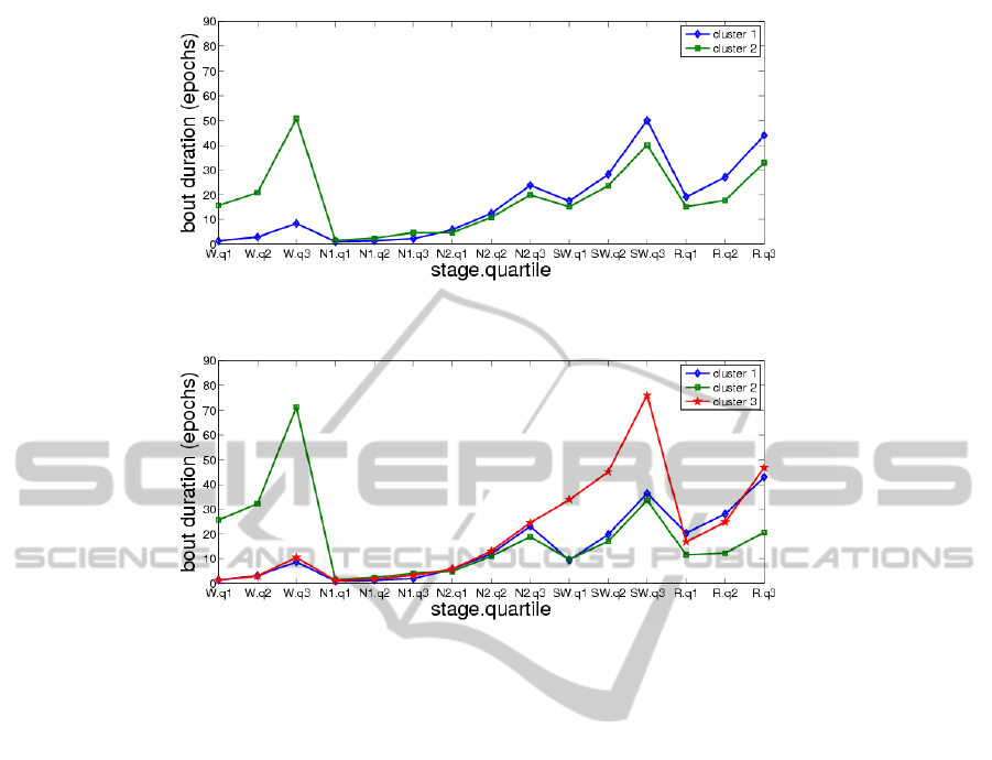
Figure 5: Mean values of clustering variables, k = 2.

Figure 6: Mean values of clustering variables, k = 3.

ter 3. See Fig. 5, Fig. 6, and Fig. 7. The bout dura-

tion characteristics of cluster 1 are remarkably stable

across values of k.

Cluster 2. Cluster 2 consistently has signiﬁcantly

higher wake bout duration quartiles than any other

cluster, for k = 2, 3, 4 (Wilcoxon p < 0.02). The

single exception is the variable wake.Q1 in the case

k = 4. Low sample sizes for k = 4 clusters 2 and 4

(15 and 24, respectively) likely contribute to the latter

isolated nonsigniﬁcance ﬁnding. One also observes

that, in the progression from k = 2 to k = 3 to k = 4,

cluster 2 has monotonically decreasing REM bout du-

ration quartiles.

Cluster 3. As observed in section 3.3.1, 145 of the

148 instances (approximately 98%) in the k = 3 ver-

sion of cluster 3 belong to the k = 2 version of cluster

1. The remainder of the k = 2 cluster 1 instances form

the majority of the k = 3 cluster 3. Therefore, it is not

surprising that many of the bout duration quartiles for

the k = 3 version of cluster 3 are similar to those for

cluster 1. See Fig. 6 and Table 5. However, there is an

immediately noticeable difference between clusters 1

and 3 for k = 3, namely the fact that cluster 3 has vis-

ibly higher SWS bout duration quartiles than all other

clusters, including cluster 1. In other words, cluster

3 for k = 3 consists mainly of those k = 2 cluster 1

instances with higher SWS bout duration quartiles.

This high SWS bout duration description of cluster 3

persists for k = 4. However, the observed SWS quar-

tile bout durationsfor cluster 3, though highest among

all clusters, are not signiﬁcantly higher than those of

clusters 2 and 4, again due likely to the small sizes of

the latter clusters.

Cluster 4. Cluster 4 is characterized by signiﬁ-

cantly higher REM bout quartile durations than any

other cluster (Wilcoxon p < 10

−3

Clustering Description via Classiﬁcation Rules.

One can compare the characterizations of the clusters

described in the preceding paragraphs with the model

constructed by the JRIP conjunctive rule classiﬁer in

the case k = 3. The model is as shown in Fig. 8, and

achieves a classiﬁcation accuracy of 0.86 and mean

ROC area of 0.88. The rules of this model closely

agree with the descriptions provided above.

MACHINE LEARNING OF HUMAN SLEEP PATTERNS BASED ON STAGE BOUT DURATIONS

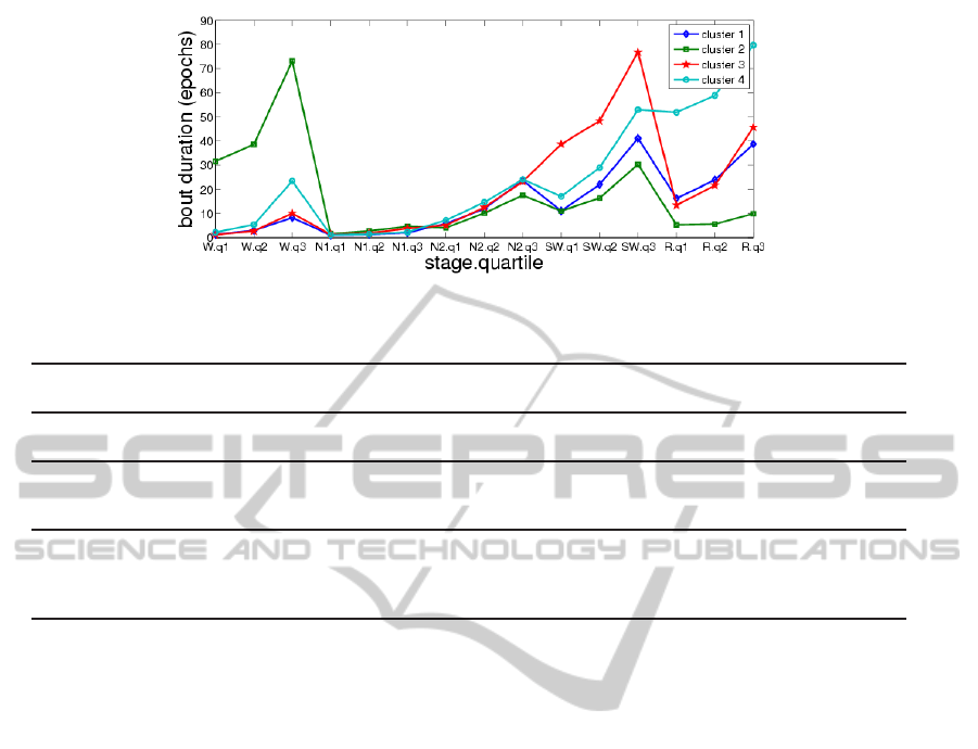
Figure 7: Mean values of clustering variables, k = 4.

Table 5: Mean bout duration quartiles of different clusters, in epochs.

wake N1 N2 SWS REM

Q1 Q2 Q3 Q1 Q2 Q3 Q1 Q2 Q3 Q1 Q2 Q3 Q1 Q2 Q3

k = 2 cluster 1 (n=211) 1.4 2.9 8.4 1.1 1.4 2.2 5.9 12 24 17 28 50 19 27 44

k = 2 cluster 2 (n=33) 16 21 51 1.5 2.5 4.6 4.6 11 20 15 24 40 15 18 33

k = 3 cluster 1 (n=148) 1.5 3.1 8.6 1.0 1.3 2.0 5.8 12 23 9.4 20 36 20 28 43

k = 3 cluster 2 (n=19) 26 32 71 1.5 2.5 4.1 4.8 11 19 9.7 17 34 12 12 21

k = 3 cluster 3 (n=77) 1.4 3 10 1.2 1.8 3.3 5.8 13 25 34 45 76 17 25 47

k = 4 cluster 1 (n=157) 1.4 3.0 8.2 1.1 1.4 2.1 5.8 12.0 24 11 22 41 16 24 39

k = 4 cluster 2 (n=15) 32 39 73 1.6 2.7 4.6 4.1 10 18 11 16 30 5.3 5.6 9.9

k = 4 cluster 3 (n=48) 1.3 2.8 10 1.2 1.9 3.7 5.1 13 23 39 48 77 13 22 46

k = 4 cluster 4 (n=24) 2.2 5.4 23 1.1 1.5 2.3 7.2 15 24 17 29 53 52 59 80

3.4 Health-related Cluster Differences

3.4.1 Comparisons of Sleep-related and

Health-related Variables

The boutduration clusters identiﬁed by the EM proce-

dure were examined to determine differences among

them in the values of sleep-related and health-related

variables not used in the clustering procedure itself.

Group comparisons of means and medians were per-

formed using ANOVA and Kruskal-Wallis tests, re-

spectively. Pairwise comparisons of means and medi-

ans used a t-test and Wilcoxon rank sum test. For all

values of k = 2, 3, 4, Kruskal-Wallis and ANOVA de-

termined that mean sleep latency (time elapsed from

getting in bed until ﬁrst non-wake epoch) differs sig-

niﬁcantly among bout duration clusters (p < 0.05).

The highest mean value of sleep latency occurs in

cluster 2. The pairwise difference in mean and median

sleep latency between cluster 2 and all other clusters

is also signiﬁcant (p < 0.05). As observed in Table 5

and discussed in section 3.3.4, cluster 2 has the high-

est mean wake bout duration quartiles of all of the

clusters. It is entirely possible that the high sleep la-

tency contributesto the increased wake bout durations

in cluster 2. Certain variables that correspond to indi-

vidual items in the EpworthDaytime Sleepiness ques-

tionnaire are also signiﬁcantly different in a multi-

way comparison among clusters, and are signiﬁcantly

different in pairwise comparisons between cluster 2

and the others in particular: a sensation of muscular

weakness or paralysis during laughter, anger, or emo-

tional situations, and the recollection of vivid dreams

and nightmares, differ signiﬁcantly among clusters

for k = 2, 3, and are highest in cluster 2 for k = 2, 3

(p < 0.05); an uncomfortable crawly sensation in the

legs that is relieved by walking differs signiﬁcantly

(p < 0.05) among clusters for k = 3, 4, and is lowest

in cluster 2.

3.4.2 Comparison with Multivariate Linear

Regression

Based on the ﬁnding of signiﬁcant differences in

health variables in section 3.4.1, it is natural to ask

whether standard linear regression can provide good

predictions of one of these variables, such as a muscle

weakness or paralysis in emotional situations, based

on bout duration statistics. In the case k = 3, least

squares linear regression yields the model in Fig. 9

(coefﬁcients shown to two signiﬁcant digits).

Terms involving wake bout duration quartiles,

which as discussed in section 3.3.3 differentiate clus-

ter 2 from the others, and in which paralysis attains

its maximum value as discussed in section 3.4.1, ap-

pear in the regression model of Fig. 9. However,

HEALTHINF 2012 - International Conference on Health Informatics

(wake.Q3 >= 44) => cluster=cluster2 (12.0/1.0)

(wake.Q2 >= 6) and (SWS.Q1 <= 5) => cluster=cluster2 (5.0/1.0)

(NREM1.Q2 >= 3) and (NREM2.Q2 <= 9) => cluster=cluster2 (5.0/1.0)

(SWS.Q1 >= 30) => cluster=cluster3 (41.0/2.0)

(NREM1.Q3 >= 4) => cluster=cluster3 (22.0/1.0)

(SWS.Q3 >= 79) => cluster=cluster3 (15.0/3.0)

(SWS.Q2 >= 49) => cluster=cluster3 (5.0/2.0)

=> cluster=cluster1 (139.0/0.0)

Figure 8: JRIP conjunctive rule model of the clusters for k = 3.

paralysis =

-0.015 wake.Q1 + 0.012 wake.Q2 + 0.0037wake.Q3

-0.22 NREM1.Q1 + 0.07 NREM1.Q3

+0.03 NREM2.Q1 + 0.018 NREM2.Q2

-0.0045 REM.Q1 - 0.012

Figure 9: Least squares linear regression model of paralysis

< 0.01).

the linear correlation between paralysis and the pre-

dictions of the least squares linear regression model

is less than 0.06. Thus, this model explains a frac-

tion that is less than 0.06

, which is much less than

1%, of the variance in paralysis. Nonlinear predic-

tive models obtained through regression based on the

machine learning technique of Support Vector Ma-

chines (SVM) provide slightly improvedperformance

here. In any case, the fact that paralysis differs sig-

niﬁcantly among the bout duration-based groupings

found through clustering, already shows that machine

learning can uncover structure in health-related data

that is not clearly identiﬁed by more traditional statis-

tical techniques such as linear regression.

4 CONCLUSIONS AND FUTURE

WORK

This paper has applied unsupervised machine learn-

ing to the discovery of patterns in human sleep data

based on the duration distributions of continuous

bouts in the various sleep stages. The results pre-

sented identify groups of hypnograms with distinct

bout duration properties. The differences in bout du-

rations amonggroups are shown to be statistically sig-

niﬁcant (p < 0.05), even after a correction to prevent

increased type I error due to multiple comparisons.

Each group is characterized by bout duration features

for speciﬁc sleep stages, the values of which differ

signiﬁcantly from those of other groups.

Several sleep-related and health-related variables

not used in the grouping procedure have been com-

pared across groups. Of these variables, several dis-

play signiﬁcantly different statistics in different bout

duration groups, including sleep latency and sev-

eral variables corresponding to items on the Epworth

Daytime Sleepiness questionnaire, such as muscular

weakness or paralysis associated with emotional situ-

ations, the recollection of vivid dreams or nightmares,

and an uncomfortable “crawly” sensation in the legs

that is relieved by walking. It is found that these vari-

ables are signiﬁcantly different in the bout duration

group characterized by the highest mean duration of

wake bouts. This ﬁnding provides a speciﬁc manner

in which sleep dynamics reﬂects the values of vari-

ables that are not speciﬁc to sleep. It is of interest to

further explore the importance within sleep medicine

of these bout duration groups in future work.

The results presented in this paper are based on a

highly compressed representation of the bout duration

distributions, utilizing only the three quartile values

of the cumulative bout duration distribution for each

sleep stage. It is possible that this compression limits

the capacity of the clustering technique to identify im-

portant dynamical features. Increasing the number of

quantiles provides greater representational accuracy,

but was found to also reduce stability of the cluster-

ing results. Future work should investigate alternative

representations of sleep dynamical information that

simultaneously provide important detail in the distri-

butions and stability of the machine learning results.

Additionally, the current work only considers the

duration of each bout in a given stage, without re-

gard for what stage occurs immediately afterwards.

It would be desirable to also consider the statistics of

speciﬁc stage transitions in future work. However, ac-

curate modeling of the sleep stage transition statistics

may require the use of multiple nights’ sleep data, or

ambulatory monitoring of key physiological signals.

REFERENCES

Aserinsky, E. and Kleitman, N. (1953). Regularly occurring

periods of eye motility, and concomitant phenomena,

during sleep. Science, 118(3062):273–274.

Benjamini, Y. and Hochberg, Y. (1995). Controlling the

false discovery rate: a practical and powerful ap-

proach to multiple testing. Journal of the Royal Sta-

tistical Society, Series B, 57(1):289–300.

Bianchi, M. T., Cash, S. S., Mietus, J., Peng, C.-K.,

and Thomas, R. (2010). Obstructive sleep apnea al-

MACHINE LEARNING OF HUMAN SLEEP PATTERNS BASED ON STAGE BOUT DURATIONS

ters sleep stage transition dynamics. PLoS ONE,

5(6):e11356.

Borg, I. and Groenen, P. J. F. (2005). Modern Multidimen-

sional Scaling: Theory and Applications (Springer

Series in Statistics). Springer, Berlin, 2nd edition.

Burns, J. W., Crofford, L. J., and Chervin, R. D. (2008).

Sleep stage dynamics in ﬁbromyalgia patients and

controls. Sleep Medicine, 9(6):689–696.

Bˇrezinov´a, V. (1976). Duration of EEG sleep stages in dif-

ferent types of disturbed night sleep. Postgrad Med J.,

52(603):3436.

Cohen, W. W. (1995). Fast effective rule induction. In

Twelfth International Conference on Machine Learn-

ing, pages 115–123. Morgan Kaufmann.

Dang-Vu, T., Schabus, M., Desseilles, M., Sterpenich, V.,

Bonjean, M., and Maquet, P. (2010). Functional

neuroimaging insights into the physiology of human

sleep. Sleep, 33(12):1589–603.

Danker-Hopfe, H., Schfer, M., Dorn, H., Anderer, P.,

Saletu, B., Gruber, G., Zeitlhofer, J., Kunz, D., Bar-

banoj, M.-J., Himanen, S., Kemp, B., Penzel, T.,

Rschke, J., and Dorffner, G. (2005). Percentile refer-

ence charts for selected sleep parameters for 20- to 80-

year-old healthy subjects from the SIESTA database.

Somnologie - Schlafforschung und Schlafmedizin,

9:3–14. 10.1111/j.1439-054X.2004.00038.x.

Dement, W. and Kleitman, N. (1957). The relation of eye

movements during sleep to dream activity: An objec-

tive method for the study of dreaming. Journal of Ex-

perimental Psychology, 53:339–46.

Dempster, A. P., Laird, N. M., and Rubin, D. B. (1977).

Maximum likelihood from incomplete data via the

EM algorithm. Journal of the Royal Statistical So-

ciety, Series B, 39(1):1–38.

Diekelmann, S. and Born, J. (2010). The memory function

of sleep. Nat Rev Neurosci, 11(2):114–126.

Fawcett, T. (2003). ROC graphs: Notes and practical

considerations for data mining researchers. Hewlett-

Packard Labs Technical Report HPL-2003-4.

Hall, M., Frank, E., Holmes, G., Pfahringer, B., Reutemann,

P., and Witten, I. (2009). The WEKA data mining

software: an update. SIGKDD Explor., 11(1):10–18.

Hubert, L. and Arabie, P. (1985). Comparing par-

titions. Journal of Classiﬁcation, 2:193–218.

10.1007/BF01908075.

Iber, C., Ancoli-Israel, S., Chesson, A., and Quan, S.

(2007). The AASM Manual for the Scoring of Sleep

and Associated Events: Rules, Terminology, and Tech-

nical Speciﬁcations. American Academy of Sleep

Medicine, Westchester, Illinois, USA.

Johns, M. W. (1991). A new method for measuring day-

time sleepiness: the epworth sleepiness scale. Sleep,

14(6):540–545.

Khasawneh, A., Alvarez, S. A., Ruiz, C., Misra, S., and

Moonis, M. (2011). EEG and ECG characteristics

of human sleep composition types. In Traver, V.,

Fred, A., Filipe, J., and Gamboa, H., editors, Proc.

HEALTHINF 2011, in conjunction with BIOSTEC

2011, pages 97–106. SciTePress.

Kishi, A., Struzik, Z., Natelson, B., Togo, F., and Ya-

mamoto, Y. (2008). Dynamics of sleep stage tran-

sitions in healthy humans and patients with chronic

fatigue syndrome. Am J Physiol Regul Integr Comp

Physiol., 294(6):R1980–7.

Krueger, J. M., Rector, D. M., Roy, S., Van Dongen, H.

P. A., Belenky, G., and Panksepp, J. (2008). Sleep as

a fundamental property of neuronal assemblies. Nat

Rev Neurosci, 9(12):910–919.

Lo, C.-C., Amaral, L. A. N., Havlin, S., Ivanov, P. C., Pen-

zel, T., Peter, J.-H., and Stanley, H. E. (2002). Dynam-

ics of sleep-wake transitions during sleep. Europhys.

Lett., 57(5):625–631.

Loomis, A., Harvey, E., and Hobart, G. (1937). Cerebral

states during sleep, as studied by human brain poten-

tials. J. Experimental Psychology, 21(2):127–144.

Moser, D., Anderer, P., Gruber, G., Parapatics, S., Loretz,

E., Boeck, M., Kloesch, G., Heller, E., Schmidt,

A., Danker-Hopfe, H., Saletu, B., Zeitlhofer, J., and

Dorffner, G. (2009). Sleep classiﬁcation according to

AASM and Rechtschaffen & Kales: Effects on sleep

scoring parameters. Sleep, 32(2):139–149.

Neal, R. and Hinton, G. (1998). A view of the EM algo-

rithm that justiﬁes incremental, sparse, and other vari-

ants. In Learning in Graphical Models, pages 355–

368. Kluwer Academic Publishers.

Penzel, T., Kantelhardt, J. W., Lo, C.-C., Voigt, K., and Vo-

gelmeier, C. F. (2003). Dynamics of heart rate and

sleep stages in normals and patients with sleep apnea.

Neuropsychopharmacology, 28(S1):S48–S53.

Propper, R., Christman, S., and Olejarz, S. (2007). Home-

recorded sleep architecture as a function of hand-

edness II: Consistent right- versus consistent left-

handers. J Nerv Ment Dis., 195(8):689–692.

Rand, W. M. (1971). Objective criteria for the evaluation of

clustering methods. Journal of the American Statisti-

cal Association, 66(336):846–850.

Rao, M., Blackwell, T., Redline, S., Stefanick, M., Ancoli-

Israel, S., and Stone, K. (2009). Association between

sleep architecture and measures of body composition.

Sleep, 32(4):483–90.

Rechtschaffen, A. and Kales, A., editors (1968). A Manual

of Standardized Terminology, Techniques, and Scor-

ing System for Sleep Stages of Human Subjects. US

Department of Health, Education, and Welfare Public

Health Service – NIH/NIND.

Storch, E. A., Roberti, J. W., and Roth, D. A. (2004). Factor

structure, concurrent validity, and internal consistency

of the Beck depression inventory–second edition in a

sample of college students. Depression and Anxiety,

19(3):187–189.

Sulekha, S., Thennarasu, K., Vedamurthachar, A., Raju,

T., and Kutty, B. (2006). Evaluation of sleep archi-

tecture in practitioners of Sudarshan Kriya yoga and

Vipassana meditation. Sleep and Biological Rhythms,

4(3):207–214.

Zhang, L., Samet, J., Caffo, B., and Punjabi, N. (2006).

Cigarette smoking and nocturnal sleep architecture.

Am J Epidemiol., 164(6):529–537.

HEALTHINF 2012 - International Conference on Health Informatics