
AUTOMATIC ESTIMATION OF MULTIPLE MOTION FIELDS
USING OBJECT TRAJECTORIES AND OPTICAL FLOW
Manya V. Afonso, Jorge S. Marques and Jacinto C. Nascimento
Instituto de Sistemas e Rob´otica, Instituto Superior T´ecnico, Lisbon, Portugal
Keywords:
Vector fields, Video segmentation, Optical flow, Trajectories.
Abstract:
Multiple motion fields are an efficient way of summarising the movement of objects in a scene and allow an
automatic classification of objects activities in the scene. However, their estimation relies on some kind of
supervised learning e.g., using manually edited trajectories. This paper proposes an automatic method for the
estimation of multiple motion fields. The proposed algorithm detects multiple moving objects and their veloc-
ities in a video sequence using optical flow. This leads to a sequence of centroids and corresponding velocity
vectors. A matching algorithm is then applied to group the centroids into trajectories, each of them describing
the movement of an object in the scene. The paper shows that motion fields can be reliably estimated from the
detected trajectories leading to a fully automatic procedure for the estimation of multiple motion fields.
1 INTRODUCTION
Video surveillance systems aim to detect and track
moving objects (e.g., pedestrians), and to character-
ize their behaviors in the scene. Surveillance sys-
tems should be able to learn typical behaviors from
video data in an unsupervised fashion, without us-
ing specific knowledge about the actions performed
by humans in the monitored environment. Such sys-
tems typically involve the following steps: (a) de-
tection of moving objects; (b) extraction of informa-
tive features (e.g. position, motion, shape); (c) track-
ing of the extracted features; and (d) classification of
the observed behavior based on the extracted features
(Turaga et al., 2008).
In outdoor applications, the object trajectories
play an important role since they allow the system
to characterize typical behaviors and discriminate ab-
normal ones. One way of modeling trajectories is
the recently proposed approach using multiple mo-
tion fields, each representing a specific type of mo-
tion(Nascimento et al., 2009). The estimation of the
motion fields is done automatically once we have a
set of trajectories containing all typical activities in
the scene. This model was applied with success to
several problems. However, the training trajectories
were hand edited to compensate for object detection
and tracking errors.
This paper aims to overcome this difficulty. It
proposes an automatic object tracking algorithm and
its application to the estimation of multiple motion
fields. The goal is to automate the estimation of mul-
tiple motion fields from the video stream.
The paper is organized as follows. Section 2, de-
scribes related work in this area. Section 3, presents
the proposed automatic trajectory extraction algo-
rithm. Section 4, describes the comparison between
the detected trajectories and manually extracted ones,
used as ground truth. Experimental results with real
data are presented in Section 5.
2 RELATED WORK
2.1 Segmentation
Segmentation is a key step in most video surveillance
systems. It aims to detect objects of interest in the
video stream, using their visual and motion proper-
ties. It plays a key role since it reduces the amount
of information to be processed by higher processing
levels and locates the position of the targets. There is
a large spectrum of segmentation methods that can be
broadly classified into the following classes: (i) statis-
tical approaches, (ii) non-statistical approaches, and
(iii) spatio-temporal approaches.
The methods of the first class adopt statistical
models for the background image, e.g., each pixel of
the background is modeled as a Gaussian distribution
457
Afonso M., Marques J. and Nascimento J. (2012).
AUTOMATIC ESTIMATION OF MULTIPLE MOTION FIELDS USING OBJECT TRAJECTORIES AND OPTICAL FLOW.
In Proceedings of the 1st International Conference on Pattern Recognition Applications and Methods, pages 457-462
DOI: 10.5220/0003783404570462
Copyright
c
SciTePress

(Wren et al., 1997) or a mixture of Gaussians (Stauf-
fer et al., 2000; McKenna and Gong, 1999). Also,
minimization of Gaussian differences has been used
(Ohta, 2001). Dynamic belief network (Koller et al.,
1994) is another type of statistical method. This class
of works also comprises a combination of frame dif-
ferences and statistical background models (Collins
et al., 1999).
Non-statistical based approaches adopt determin-
istic descriptions of the background image. The
simplest approach is called background subtraction
method, in which, a pixel-wise difference between
the current frame and the background model is per-
formed. Foreground/backgorund pixels are deter-
mined if the resulting difference is above/under a
pre-determined threshold, respectively (Gonzalez and
Woods, 2002). Other methods consider an admis-
sible range for each pixel intensity, maximum rate
of change in consecutive images or the median of
largest inter-frames absolute difference (Haritaoglu
et al., 2000).
The third class is based on spatio-temporal seg-
mentation of the video signal. These methods try to
detect moving regions taking into account not only the
temporal evolution of the pixel intensities and color
but also their spatial properties. Segmentation is per-
formed in a 2D+T region of image-time space, con-
sidering the temporal evolution of neighboring pix-
els. This can be done in several ways, e.g. by using
spatio-temporal entropy (Ma and Zhang, 2001), or the
3D structure tensor defined from the pixels spatial and
temporal derivatives (Souvenir et al., 2005).
2.2 Optical Flow
Optical flow is a measure of the apparent motion of
all image pixels from one frame to the next. With
some exceptions, it is an estimate of the motion field
(Barron et al., 1994), (Simoncelli, 1993). Denoting
the image intensity at position (x, y) and time t by
I(x, y,t), the optical flow equation is
(∇
x
I)(x, y,t)u+ (∇
y
I)(x, y,t)v+ (∇
t
I)(x, y,t) = 0,
(1)
where x, y indicates a pixel location, and ∇
x
I, ∇
y
I, and
∇
t
I respectively denote the image gradient along the
x, y and t directions. This equation is not enough to
obtain the velocity vector (u, v) associated to each im-
age point since it has an infinite number of solutions.
This is known as the aperture problem. Additional
constraints like smoothness have to be used.
There are several methods for computing the
optical flow. Gradient based methods that im-
pose smoothness constraints on the field of veloc-
ity vectors, the Horn and Schunck method (Horn
and Schunck, 1981) that uses a global smoothness
constraint or the Lucas-Kanade method (Lucas and
Kanade, 1981) that assumes the velocity is locally
constant combining local constraints over local re-
gions. These methods are considered more accurate
than the ones based on template matching, but they
can only be used if the displacements is small (Bar-
ron et al., 1994).
There are several ways to deal with large displace-
ments. One approach is region-matching based meth-
ods which do not actually solve (1), but try to find the
most likely position for an image region in the next
frame. Yet, another method is the Bayesian multi-
scale coarse to fine algorithm (Simoncelli, 1993). A
coarse to fine warping scheme involving two nested
fixed point iterations for energy minimization func-
tional was proposed in (Brox et al., 2004) and a vari-
ant of this method (Sand and Teller, 2008), wherein
video motion is represented by a set of particles and
particle trajectories yielding the displacements as well
as trajectories representing their motion.
2.3 Multiple Motion Field Model
Multiple motion fields were recently proposed as a
tool to summarize objects motion in a scene and
to statistically characterize their trajectories (Nasci-
mento et al., 2009). Each trajectory is assumed to be
a sequence of segments, each of them being generated
by one of the motion fields, the so-called active field.
Model switching is performed based on a probabilis-
tic mechanism whose parameters depend on the posi-
tion of the object in the image. This model is flexible
enough to represent a wide variety of trajectories and
allows the representation of space-varying behaviors
as required.
Each trajectory is a length-n sequence of positions
x = (x
1
, ..., x
n
) with x
t
∈ R
2
. Each position represents
the centroid of the object in the image. We assume
each trajectory is the output of a switched dynamical
system
x
t
= x
t−1
+ T
k
t
(x
t−1
) + w
t
, (2)
where k
t
∈ {1, . . . , M} is the label of the active field
at time t; {T
1
, . . . , T
M
} are M vector fields which de-
scribe typical motion patterns and (w
1
, . . . , w
n
) are in-
dependent samples of a zero-mean Gaussian random
vector with identity covariance.
The label sequence k = (k
1
, ..., k
n
) is assumed to
be a Markov chain of order one with space-dependent
transition probabilities
Pr{k
t
= j|k
t−1
= i, x
t−1
} = b
ij
(x
t−1
) (3)
Matrix B(x
t−1
) = (b
ij
(x
t−1
)) is a space-varying
stochastic matrix. The model parameters (motion
ICPRAM 2012 - International Conference on Pattern Recognition Applications and Methods
458

fields, noise variances, switching matrix field) can be
retrieved from observed object trajectories using the
Expectation-Maximization (EM) algorithm.
3 PROPOSED APPROACH
In this section, we describe the segmentation and fea-
ture extraction processes. We first perform back-
ground subtraction to detect the active regions in a
frame, and then estimate the velocity fields at the cen-
troid of each active region by computing the optical
flow using the template matching algorithm. The re-
sult of these steps is a sequence of vectors containing
the spatial coordinates of the centroids of the active
regions, over the entire set of frames, and also the cor-
responding velocity fields.
3.1 Active Region Detection
We represent a frame at time t with M rows and N
columns by a matrix I
t
∈ R
M× N
. Given a sequence
of K frames { I
t
,t = 1, ..., K}, we estimate the back-
ground image B ∈ R
M× N
by taking a subset of frames
and applying a median filter to the evolution of each
pixel in time. We segment each frame I
t
, by subtract-
ing the background and thresholding the difference
image with a predefined positive value λ, to produce
a binary image J
t
∈ { 0, 1}
M× N
with the value at pixel
m, n,
J
t
(m, n) =
1, if |I
t
(m, n) − B(m, n)| > λ,
0, otherwise.
(4)
For multiple moving objects, this requires finding the
connected pixels above this threshold. We do not as-
sume beforehand, the number of moving objects. We
therefore apply a clustering algorithm on this binary
image J
t
to find connected regions (assuming 8 neigh-
bors), each cluster corresponding to a moving object.
In practice, because of the empirical nature of the
threshold value λ, there may be false active regions
(i.e. the threshold being exceeded where there is no
motion) or the active region corresponding to a single
moving object may get split into two or more clus-
ters. We solve the second problem by dilating the bi-
nary image J
i
before clustering, and solve the prob-
lem of false active regions by discarding the clusters
with small area. The number of active regions de-
tected at the frame t,will be denoted by n
t
.
3.1.1 Optical Flow using Template matching
Region based matching approaches for computing the
optical flow define the velocity vector of an object
moving across successive frames as the vector of dis-
placements (i, j) that produces the best fit between
image regions at different times. The best fit means
that a distance measure between a region in a frame,
I
t
, and its possible location in the next frame, I
t+1
, is
minimum for the vector (i, j), or a similarity measure
such as cross-correlation is maximum. These meth-
ods are intuitively simple and relatively easy to im-
plement, and the computational load is low since it
has to be computed only for the active regions.
Let the bounding box of the k − th active region
be I
k
∈ Z
2
. Then assuming suitable boundary condi-
tions, the velocity vector is computed by solving the
optimization problem,
(u
k
, v
k
) = arg min
(i, j)∈(−d
m
,d
m
)
E(i, j), (5)
E(i, j) =
∑
(m,n)∈I
k
(I
t
(m, n)−I
t+1
(m+i, n+ j))
2
+α(|i|+| j|).
(6)
where d
m
is the maximum displacement, and α > 0
is the regularization parameter that controls the rela-
tive weight of the penalty term. Since the entire block
is assumed to be displaced by the vector (u
k
, v
k
), we
consider this the optical flow at the centroid of the k
th
region.
Figure 1 illustrates the optical flow between two
frames at times t and t + 1, for a man walking. The
velocity vector is shown superimposed over the frame
at time t and its binary image, at the centroid of the
active region corresponding to the man.
Figure 1: Optical flow between 2 frames. (a),(b) grayscale
frames at times t and t + 1, (c), (d) active regions corre-
sponding to the moving person in the two frames.
3.2 Motion Correspondence
At the end of the optical flow step, we have a set of
n
t
centroid locations {(x
i
, y
i
), i = 1, ..., n
t
} and their
respective motion vectors {(u
i
, v
i
), i = 1, ..., n
k
}. We
therefore need to apply a region association algorithm
to integrate the centroids in successive frames into tra-
jectories. This differs from the approach presented in
(Nascimento et al., 2010), where the pre-processing
consists of two steps: active region detection using
the Lehigh Omnidirectional Tracking System (LOTS)
algorithm followed by region association. The ap-
proach herein proposed is threefold regarding the pre-
processing in [Nascimento et al., 2010]: (1) it com-
putes directly the vector fields, (2) it reduces drasti-
cally the errors that may arise in the region associa-
tion mechanism, and (3) consequently avoids manual
AUTOMATIC ESTIMATION OF MULTIPLE MOTION FIELDS USING OBJECT TRAJECTORIES AND OPTICAL
FLOW
459

corrections to obtain the trajectories. In this paper,
we directly apply a motion correspondencealgorithm,
namely, the GOA tracker (Veenman et al., 2001) on
the sequence of centroid positions.
Let the vector x
t
k
= [x
k
, y
k
]
T
denote the position
vector of the centroid of active region k in frame t. For
the centroids of two regions i and j in two successive
frames t and t + 1, the association cost is
C
t
(i, j) = kx
t+1
j
− (x
t
i
+ v
t
i
)k
2
, (7)
where v
t
k
= [u
k
, v
k
]
T
is the velocity vector at the cen-
troid of active region k in frame t.
Let
˜
C
t
be the size n
t+1
× n
t
matrix whose entries
are computed using the above cost function. In gen-
eral, the number of centroids in successive frames is
not the same, that is, n
t+1
6= n
t
. A centroid in frame t
may have a correspondingpoint in framet+1 belong-
ing to its trajectory or it may be the last point belong-
ing to that particular trajectory. Likewise, a centroid
in frame t + 1 may belong to a trajectory having an
associated point in frame t, or it could be the starting
point of a new trajectory. To be able to account for
the “birth” or “death” of trajectories, we pad the ma-
trix
˜
C
t
with entries equal to γ to form a square cost
matrix C
t
of size (n
t
+ n
t+1
) × (n
t
+ n
t+1
),
C
t
=
˜
C
t
, γ1
(n
t+1
×n
t+1
)
γ1
(n
t
×n
t
)
, γ1
(n
t
×n
t+1
)
, (8)
where 1 stands for a matrix whose entries are all 1,
γ > 0 is the cost of starting a new trajectory or end-
ing an existing one. A column of this matrix corre-
sponds to a centroid in frame t and a row corresponds
to a centroid in frame t + 1. The Hungarian match-
ing algorithm (Kuhn, 1955) is then used to solve the
matching problem by minimizing the assignment cost
C =
n
t
+n
t+1
∑
i, j=1
b
ij
C
ij
, (9)
where b
ij
∈ {0, 1} and have the constraints
n
t
+n
t+1
∑
i=1
b
ij
= 1, ∀ j ;
n
t
+n
t+1
∑
j=1
b
ij
= 1, ∀ i . (10)
4 COMPARISON WITH GROUND
TRUTH
Once we have computed a trajectory of an object in
a given video sequence as described in the previous
section, we would like to compare it with the trajec-
tory for the same object from the set of previously
computed trajectories which we consider the ground
truth. We would like to do this automatically, without
the user having to manually locate the sequence of
frames corresponding to the trajectory. This has the
possible problems that the trajectory and its counter-
part from the ground truth may not exactly coincide in
terms of starting and ending frames, may have some
missed detections in some frames, or a single trajec-
tory may have multiple trajectories in the ground truth
corresponding to different segments (e.g. an object
moving in loops).
We denote an automatically detected trajectory
by {x}
t∈T
, defined over a subset of frames T =
{t
0
, . . . , t
M
}. Similarly, a trajectory i from the ground
truth set is denoted as {x
gt,i
}
t∈T
i
, with T
i
being the
set of relevant frames. If there are some frames in
common between T and T
i
, we define the set of over-
lapping frames, T
OL,i
= T ∩ T
i
, and compute the mean
square error between the two trajectories at the times
corresponding to the overlapping frames
E(i) =
1
#T
OL,i
∑
t∈T
OL,i
kx
t
− x
gt,i
t
k
2
. (11)
We then find all trajectories in the ground truth for
which the MSE is within a limit of κ times the mini-
mum value, E
min
, {i : E(i) ≤ κE
min
}. From this set,
the trajectories which have no overlapping frames are
the ones corresponding to different continuous seg-
ments of the trajectory {x}
t
.
5 EXPERIMENTAL RESULTS
We illustrate our proposed approach on a set of video
sequences of a university campus (Instituto Superior
T´ecnico, Lisbon) recorded with a single static cam-
era. The total number of frames was 69596, acquired
at a rate of 25 frames per second. For our compu-
tation of optical flow, the sequence was subsampled
at a rate of 5 frames. The frame size is 432× 540.
There were 7 pedestrian activities of interest in this
sequence, which are listed in Table 1.
Figure 2 shows two trajectories corresponding to
people walking, detected over a segment of 2000
frames, and their respective velocity vectors superim-
posed. The velocities were scaled by a factor of 10
and subsampled by a factor of 8 for display.
Figure 3 shows the two trajectories from Figure 2
and the corresponding ground truth trajectories, re-
trieved by the library search. The trajectory in Fig-
ure 3(a) corresponds to a single trajectory from the
ground truth library. The other trajectory of a person
leaving the building and entering it again, which ap-
pears as a loop in Figure 3(b) has two non-overlapping
matches in the ground truth (corresponding to activi-
ties “entering” and “leaving”), which are 70 frames
ICPRAM 2012 - International Conference on Pattern Recognition Applications and Methods
460
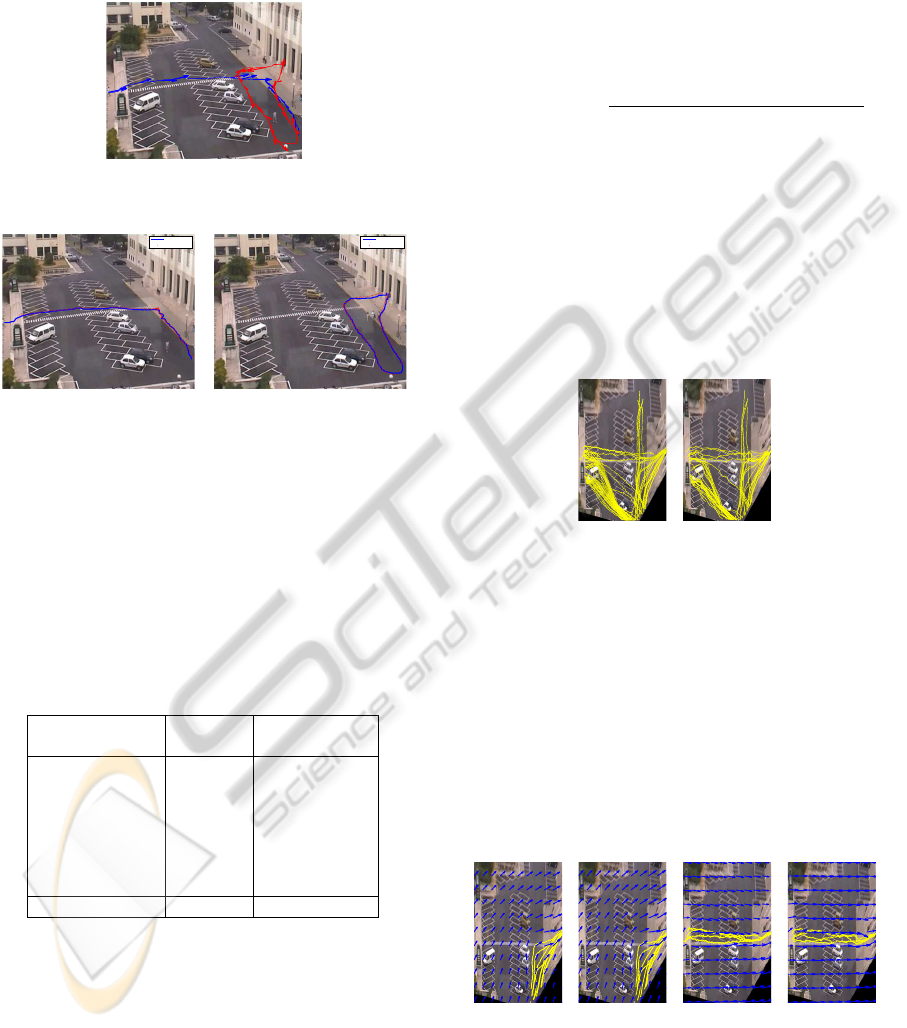
apart. Therefore, for the estimation of the motion
fields using the EM algorithm, we split this trajectory
into two segments corresponding to the two ground
truth trajectories for these activities.
Figure 2: Motion fields computed using optical flow super-
imposed over the corresponding trajectories.
Estimated
Ground Truth
(a)
Estimated
Ground Truth
(b)
Figure 3: Extracted trajectories using the proposed ap-
proach and their corresponding ground truth trajectories.
We validate our method by computing the statis-
tics of the root mean square error (RMSE) between
the trajectories obtained using our method and the
ground truth trajectories from (Nascimento et al.,
2010). We present the mean and variance of the er-
ror for each class of activities and overall values, in
Table 1.
Table 1: Statistics of the Error in the Trajectories.
Trajectory class Error Mean Error Standard
(pixels) Deviation (pixels)
entering 4.03 0.99
leaving 3.80 1.07
walking along 2.46 0.35
crossing park up 4.12 1.29
crossing park down 5.33 1.80
passing through cars 4.49 0.87
browsing 3.23 0.82
Overall 4.31 1.59
We also validate the trajectories by estimating
the motion fields from the model (2) with parame-
ters estimated by the EM method (Nascimento et al.,
2009). It is not possible to directly compare the vec-
tor fields obtained from both sets of trajectories since
the field estimates depend on the initialization of the
EM method. We therefore, evaluated each set of vec-
tor fields by measuring its ability to predict the target
position at the next time instant. For this dynamic
model, the predictor and prediction error are given by
ˆ
x
t
= x
t−1
+ T
k
t
(x
t−1
), (12)
ˆ
e
t
= x
t
− x
t−1
− T
k
t
(x
t−1
). (13)
In practice, we do not know the active field k
t
, and
therefore select the error with the smallest norm (ideal
switching). We can now define an SNR measure
SNR = 10log
10
∑
L
t=2
kx
t
− x
t−1
k
2
∑
L
t=2
min
k
kx
t
− x
t−1
− T
k
(x
t
)k
2
.
(14)
The same number of trajectories per activity was
used to train the model for both the ground truth and
our extracted trajectories, with a total of 69 trajecto-
ries. Figure 4 shows both sets of trajectories after ap-
plying a projective transformation (homography) be-
tween the image and a plane parallel to the ground.
This is done to achieve viewpoint invariance, by pro-
jecting all image measurements onto a view orthogo-
nal to the ground plane (the so-called birds eye view).
(a) (b)
Figure 4: Trajectories from (a) the ground truth and (b) ob-
tained using the proposed approach, superimposed on the
starting frame, after applying a homography.
Figure 5 shows the motion fields estimated us-
ing the EM algorithm, trained with trajectories corre-
sponding to a single activity, with one model. Figures
5(a) and 5(b) show the motion fields for the activity
“entering” using the trajectories from the ground truth
set, and those obtained using the proposed approach,
respectively. Similarly, Figures 5(a) and 5(b) present
the corresponding motion fields for the activity “pass-
ing through cars”.
(a) (b) (c) (d)
Figure 5: Motion fields for the activities “Entering” and
“Passing through cars”, estimated from (a),(c) the GT tra-
jectories, and (b),(d) extracted trajectories.
Table 2 shows the best SNRs obtained for the
AUTOMATIC ESTIMATION OF MULTIPLE MOTION FIELDS USING OBJECT TRAJECTORIES AND OPTICAL
FLOW
461

Table 2: SNR between the trajectory and predicted trajectory from the estimated motion fields.
No. of models 1 2 3 4 5 6 7 8
Ground truth 1.37 4.57 4.09 6.23 5.62 5.4 5.48 3.58
Proposed method 1.15 4.42 4.13 6.02 5.52 3.45 5.05 2.96
ground truth trajectories (corresponding to all activi-
ties) and those obtained using the proposed approach
for different numbers of fields estimated by the EM
algorithm. It can be seen that the maximum SNR ob-
tained from the extracted trajectories is close to that
obtained from the ground truth data.
6 CONCLUSIONS
We have proposed a method for automatically com-
puting the trajectories and velocity fields of multi-
ple moving objects in a video sequence, using opti-
cal flow. The trajectories obtained were found to be
close to the manually edited ground truth trajectories,
for a large set of activities occurring in the video se-
quences. The motion fields estimated from these tra-
jectories using the EM method led to an SNR close
to that obtained with the ground truth trajectories.
Hence the proposed method allows fully automatic
extraction of multiple motion fields. Current and fu-
ture work includes extending the method to denser en-
vironments such as crowds of moving people.
ACKNOWLEDGEMENTS
This work was supported by Fundac¸
˜
ao para a
Ci
ˆ
encia e Tecnologia (FCT), Portuguese Ministry
of Science and Higher Education, under projects
PTDC/EEA-CRO/098550/2008 and PEst-OE/EEI/
LA0009/ 2011.
REFERENCES
Barron, J. L., Fleet, D. J., and Beauchemin, S. S. (1994).
Performance of optical flow techniques. International
Journal of Computer Vision, 12:43–77.
Brox, T., Bruhn, A., Papenberg, N., and Weickert, J. (2004).
High accuracy optical flow estimation based on a the-
ory for warping. In ECCV (4), pages 25–36.
Collins, R., Lipton, A., and Kanade, T. (1999). A sys-
tem for video surveillance and monitoring. In Proc.
American Nuclear Society (ANS) Eighth Int. Topical
Meeting on Robotic and Remote Systems, pages 25–
29, Pittsburgh, PA.
Gonzalez, R. C. and Woods, R. E. (2002). Digital Image
Processing. Prentice Hall.
Haritaoglu, I., Harwood, D., and Davis, L. S. (2000). W
4
:
real-time surveillance of people and their activities.
22(8):809–830.
Horn, B. K. P. and Schunck, B. G. (1981). Determining
optical flow. Artificial Intelligence, 17:185–203.
Koller, D., Weber, J., Huang, T., Malik, J., Ogasawara, G.,
Rao, B., and Russel, S. (1994). Towards robust auto-
matic traffic scene analysis in real-time. In Proc. of
Int. Conf. on Pat. Rec., pages 126–131.
Kuhn, H. (1955). The Hungarian method for the assign-
ment problem. Naval research logistics quarterly,
2(1-2):83–97.
Lucas, B. D. and Kanade, T. (1981). An iterative image
registration technique with an application to stereo vi-
sion. pages 674–679.
Ma, Y.-F. and Zhang, H.-J. (2001). Detecting motion ob-
ject by spatio-temporal entropy. In IEEE Int. Conf. on
Multimedia and Expo, Tokyo, Japan.
McKenna, S. J. and Gong, S. (1999). Tracking colour ob-
jects using adaptive mixture models. Image Vision
Computing, 17:225–231.
Nascimento, J., Figueiredo, M., and Marques, J. (2009).
Trajectory analysis in natural images using mixtures
of vector fields. In IEEE Int. Conf. on Image Proc.,
pages 4353 –4356.
Nascimento, J., Figueiredo, M., and Marques, J. (2010).
Trajectory classification using switched dynamical
hidden markov models. IEEE Trans. on Image Proc.,
19(5):1338 –1348.
Ohta, N. (2001). A statistical approach to background sup-
pression for surveillance systems. In Proc. of IEEE
Int. Conf. on Computer Vision, pages 481–486.
Sand, P. and Teller, S. (2008). Particle video: Long-range
motion estimation using point trajectories. Int. J.
Comput. Vision, 80:72–91.
Simoncelli, E. P. (1993). Course-to-fine estimation of vi-
sual motion. In IEEE Eighth Workshop on Image and
Multidimensional Signal Processing.
Souvenir, R., Wright, J., and Pless, R. (2005). Spatio-
temporal detection and isolation: Results on the
PETS2005 datasets. In Proceedings of the IEEE
Workshop on Performance Evaluation in Tracking and
Surveillance.
Stauffer, C., Eric, W., and Grimson, L. (2000). Learn-
ing patterns of activity using real-time tracking.
22(8):747–757.
Turaga, P., Chellappa, R., Subrahmanian, V., and Udrea, O.
(2008). Machine recognition of human activities: A
survey. Circuits and Systems for Video Technology,
IEEE Transactions on, 18(11):1473 –1488.
Veenman, C., Reinders, M., and Backer, E. (2001). Resolv-
ing motion correspondence for densely moving points.
IEEE Trans. on Pattern Analysis and Machine Intelli-
gence, 23(1):54 –72.
Wren, C. R., Azarbayejani, A., Darrell, T., and Pentland,
A. P. (1997). Pfinder: Real-time tracking of the human
body. 19(7):780–785.
ICPRAM 2012 - International Conference on Pattern Recognition Applications and Methods
462
