LONG TERM BIOSIGNALS VISUALIZATION AND PROCESSING

Ricardo Gomes

, Neuza Nunes

, Joana Sousa

and Hugo Gamboa

1,2

Physics Department, FCT-UNL, Lisbon, Portugal

PLUX Wireless Biosignals S.A., Lisbon, Portugal

Keywords:

Biosignal, signal processing, Long term monitoring, Data structure.

Abstract:

Long term acquisitions of biosignals are an important source of information about the patients’ state and its

evolution, but involves managing very large datasets, which make signal visualization and processing a com-

plex task. To overcome these problems, we introduce a new data structure to manage long term biosignals.

A fast and non-speciﬁc multilevel biosignal visualization tool based on the concept of subsampling is pre-

sented, with focus on the representative signal parameters (mean, maximum, minimum and standard deviation

error). The visualization tool enables an overview of the entire signal and a more detailed visualization in

speciﬁc parts which we want to highlight. The ”Split and Merge” concept is exposed for long term biosig-

nals processing. A processing tool (ECG peak detection) was adapted for long term biosignals. Several long

term biosignals were used to test the developed algorithms. The visualization tool has proven to be faster

than the standard methods and the developed processing algorithm detected the peaks of long term ECG sig-

nals fast and efﬁciently. The non-speciﬁc character of the new data structure and visualization tool, and the

speed improvement in signal processing introduced by these algorithms makes them useful tools for long term

biosignals visualization and processing.

1 INTRODUCTION

The increasing development of medical systems and

applications for human welfare has been supported

by patients’ body signals monitoring. These biosig-

nals give the researcher or clinician a perspective over

the patient’s state since they carry information about

complex physiologic mechanisms. Biomedical signal

analysis has great importance for data interpretation

in medicine and biology.

In order to analyze the patient’s condition it is

very important to visualize the acquired signals and

extract relevant information from them. In clinical

cases such as neuromuscular diseases and sleep disor-

ders, a constant monitoring of the patient’s condition

is necessary (Pinto et al., 2010; Kayyali et al., 2008),

due to the possible occurrence of sudden alterations

in the patient’s state. However, long term acquisitions

generate large amounts of data, which exceed the ca-

pabilities for which standard analysis and processing

software were designed. In addition to the difﬁculty

of handling large amounts of data, displaying these

biosignals using standard visualization software is not

feasible due to our inability to correctly visualize the

entire signal. In a future perspective, the continuous

monitoring of biosignals will allow to know before-

hand when the patient needs assistance, assuring the

patients’ comfort as they are monitored in ambient as-

sisted living conditions (Sousa et al., 2010).

We present new tools for the visualization and pro-

cessing of very large biological datasets. The follow-

ing section presents the developed tools and the new

data structure for long term biosignals. In section 3

we present the methods of the developed work and

discuss the results and algorithm’s performance. Fi-

nally, we conclude the work in section 4.

2 PROPOSED DATA STRUCTURE

AND DEVELOPED TOOLS

As we are dealing with very long signals, a tool to

display large amounts of data is needed. Since we

used acquisition equipment that saves (raw) data in

text ﬁles, random access to a speciﬁc time window

of the recording wasn’t possible. To overcome this,

we created a new data structure that enables fast data

accessing, based on the HDF5 ﬁle format, a powerful

tool for managing different types of data (HDF group,

2007).

402

Gomes R., Nunes N., Sousa J. and Gamboa H..

LONG TERM BIOSIGNALS VISUALIZATION AND PROCESSING.

DOI: 10.5220/0003784704020405

In Proceedings of the International Conference on Bio-inspired Systems and Signal Processing (BIOSIGNALS-2012), pages 402-405

ISBN: 978-989-8425-89-8

 2012 SCITEPRESS (Science and Technology Publications, Lda.)

2.1 Long Term Biosignals Data

Structure

The data structure architecture (Figure 1) is based on

three sections: the acquisition data, the biosignals,

and the processed data. The biosignals section is com-

posed by the raw data and the different ”zoom levels”.

To obtain the different zoom levels, the four subsam-

pling parameters shown in Figure 1 are extracted from

the signal. Data mean identiﬁes its central location,

being a representative measure of the signals’ shape.

Maximum and minimum parameters deﬁne the enve-

lope on which the signal is restrained, while the stan-

dard deviation error provides information about the

signal’s spreading.

The ﬁrst (most detailed) level of visualization is

the raw data. The subsequent zoom levels provide

less detail than the preceding one, since they have a

smaller number of samples. However, they represent

the same time interval. The different zoom levels are

created by a subsampling process. Each subsampling

operation is carried out by splitting the input signal

in groups with a selected number of samples - the re-

sampling factor (r), and for each group the represen-

tative signals measures are calculated. The r factor

can be, for example 10, which means that the signal’s

measures will be computed from 10 to 10 samples.

Therefore, the data length will be divided by r, since

each group with r samples is represented by one new

sample. The ﬁrst zoom level is obtained taking the

raw data as input. For higher zoom levels, the al-

gorithm takes as input the data from the last zoom

level to be created, taking advantage of the data reduc-

tion on each iteration, since it calculates the mean of

means, the maximum of maxima, minimum of min-

ima (calculating the mean is faster for 1000 values

than for 10000). The standard deviation error, (sd), is

obtained with equation1, where E[X] is the expected

value for the random variable X.

sd(X) =

E[X − E[X]

] =

E[X] −E[X]

(1)

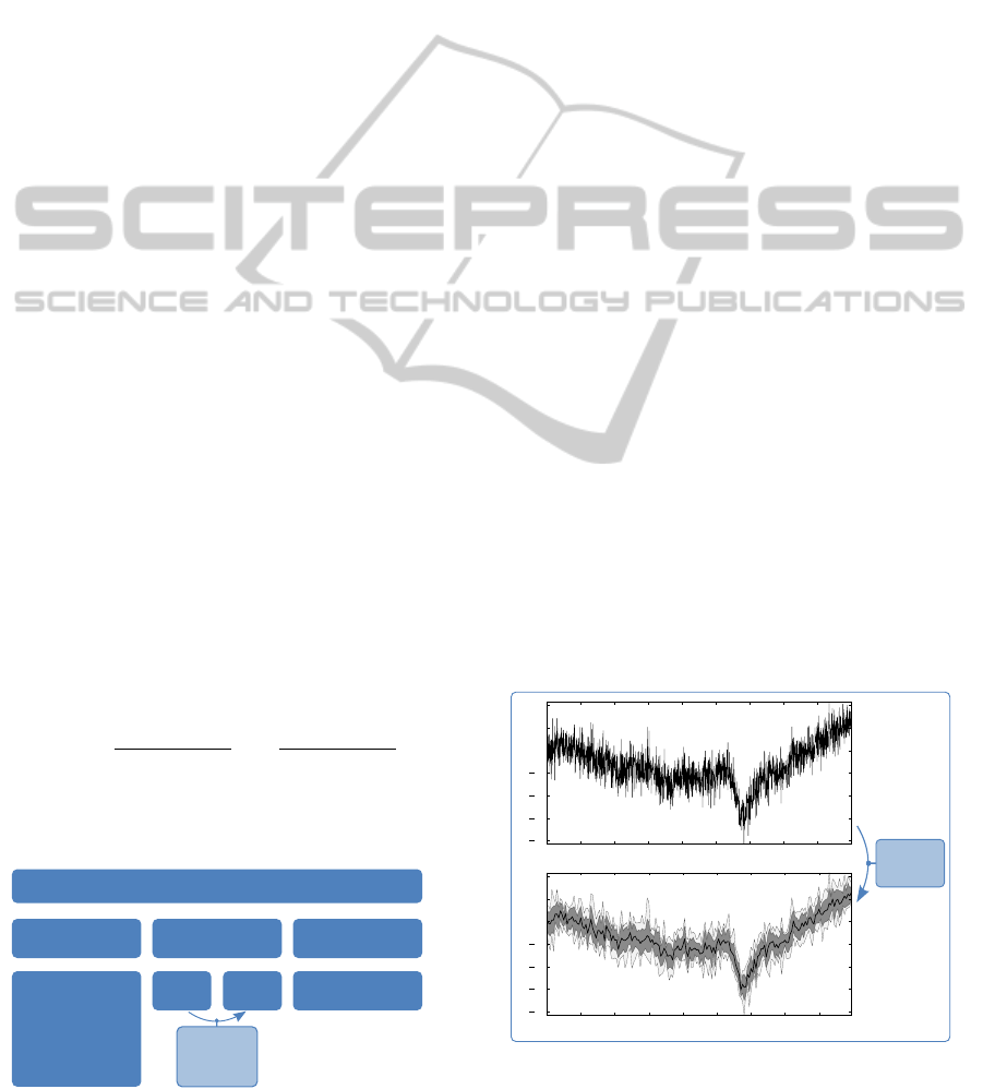
The visual effect and data mining of the described

subsampling technique are shown in Figure 2.

biosignals

visualiza

zoom

levels

raw

data

processed data

.h5 file architecture

acquisition data

- subject's name

- date

- mac address

- sampled channels

- digital channels

- recording duration

- sampling frequency

- ECG peaks

(...)

subsampling

mean

maximum

minimum

standard error

Figure 1: Proposed data structure for biosignals.

2.2 Long Term Biosignals Visualization

Based on the presented data structure, a tool to vi-

sualize long term biosignals was implemented. This

tool provides an overview of entire long term signals

in the ﬁrst instance and allows to zoom in and out

to speciﬁc time windows. This approach is compa-

rable to web mapping services, but applied to the vi-

sualization of electrophysiological signals. A client-

server model was implemented, giving the tool higher

portability, using Python as a way to manage data and

Javascript and HTML to create the visualization plat-

form. The initial display is done by drawing the entire

signal: the outermost (lowest) zoom level; the signal

being shown is updated when the navigation keys (for

zooming and panning) are pressed. Signal navigation

is facilitated by an overview window, that indicates

the selected region of the signal and enables the user

to select precise time windows in the signal to be visu-

alized in detail. There are two drawing stages which

allow a fast view of the signal’s shape:

• Preview. the signals’ informations to be drawn

are only the maximum and minimum (aiming for

a fast and representative overview);

• Detailed View. draws the signal’s mean, maxi-

mum, minimum, and the error shade (deﬁned by

mean±standard deviation error).

These drawing steps enable a faster navigation,

since the user can ask for new time windows to be

displayed almost instantly. The detailed data is shown

only when the viewer stops in a speciﬁc time window,

providing the complete information about the signal.

When the raw data level is reached, no detailed infor-

mation is shown, since there are no statistical param-

eters of the biosignal.

0 200 400 600 800 1 000 12 00 1 400 16 00 180 0

0 200 400 6 00 800 10 00 1 200 140 0 1600

180 0

subsampling

1800 samples

180 samples

Time(ms)

mean

maximum

minimum

standard error

AmplitudeAmplitude

Figure 2: Illustration of the effect produced by a subsam-

pling operation over a random signal (adimensional ampli-

tude).

LONG TERM BIOSIGNALS VISUALIZATION AND PROCESSING

403

z =



log(N)

log(r)

−

log(npviz)

log(r)

+ 1



(2)

The correct zoom level, z, corresponding to each

selected zoom window is obtained with equation 2,

where N is the number of points that we are trying to

see and npviz is the maximum number of points to be

displayed (npviz and r are speciﬁed by the user). dxe

represents the ceiling operation (rounding for the next

integer).

2.3 Long Term Biosignals Processing

Besides visualization problems, long term biosignals

also need different processing approaches. Since we

are working with very large datasets, the processing

algorithms’ input can’t be the entire signal. The im-

plemented processing algorithms map the signal in in-

tervals with ﬁxed length and process each mapped in-

terval, using an algorithm that works efﬁciently with

shorter signals. After processing each interval, the re-

sults are merged together.

X = {x

, x

, . . . , x

} (3)

Y = F(X ) (4)

Hereafter, we consider the discrete biosignal to be

processed, X, described in equation 3, where k repre-

sents the signal’s number of samples. The processing

operation can be represented by equation 4. The op-

erator F receives an entire biosignal (X) as input and

returns Y . Since the input signal might be very long,

X can be splitted in subgroups with a ﬁxed number

of samples - L. The signal mapper is a list of pairs

that deﬁne the several subgroups to be processed sep-

arately (see J in equation 5).

J = {(0, L), (L − v, L − v + L),

(2L − 2v, 2L − 2v + L),

. . . ,

(mL − mv, mL − mv + L)} (5)

v is the number of samples to be overlapped, and

m an integer. Selecting the signal (X ) in the time in-

tervals deﬁned by J, the signal will be mapped. Each

part of the signal can be deﬁned by equation 6.

= {x

, . . . , x

}

= {x

L−v

, . . . , x

L−v+L

}

··· (6)

In order to avoid problems in the borders where

the signal is splitted, the implemented algorithm has

an overlapping number of samples, v (every time the

algorithm runs for a selected time window, there is a

number of samples from the end of the last time win-

dow that is in tthe beginning of the actual one). After

mapping the signal, the processing algorithm is ap-

plied to the various intervals mapped from the signal

and a group of outputs is obtained (equation 7).

= f (x

) (7)

On this last step, in which j represents a subpro-

cessing group, the results from the independent pro-

cessing tasks are merged together. The function that

correctly joins together the outputs from the subpro-

cessing tasks is denoted by G. The ﬁnal result is given

by equation 8.

Y = G(y

, y

, . . . ) (8)

A mature algorithm (Pan and Tompkins, 1985),

which do not work properly on long term biosignals

was adapted: the ECG peak detector.

Considering a processing operation with a ﬁxed

start time (T

), that takes a time T to be carried out by

one processor and that the processing is going to be

divided by N

processors, the total parallel processing

time (T

) will be given by equation 9 (the multiplica-

tion by (1 + Ov) avoids the result to be zero).

= T

× (1 + Ov) (9)

slice

(10)

The overlap (Ov) is deﬁned by equation 10, where

slice

is the number of samples of each processing

slice. Since the existence of the overlap means that

there are samples being processed in two different

subtasks, a bigger overlap causes the processing to

last longer. However, if the overlap is too small, there

is the danger of occurring processing errors. In order

to prevent these errors, our ECG peak detection al-

gorithm only considers the data to be efﬁciently pro-

cessed when there are coincident peaks in the output

(adjacent subtasks detect at least one common peak).

3 PERFORMANCE EVALUATION

Several types of biosignals such as as electromyog-

raphy, electrocardiography, electrodermal activiy, ac-

celerometer and respiration were acquired in order to

test the visualization and processing algorithms. The

acquisitions were carried out at the patients’ homes,

with their approval, during the night (each recording

had the approximate duration of 8 hours), using a bio-

PLUX research system, a wireless signal acquisition

unit (PLUX, 2011).

BIOSIGNALS 2012 - International Conference on Bio-inspired Systems and Signal Processing

404

Table 1: Conversion times.

text ﬁle size (MB)

Conversion times (s)

raw data zoom levels

346,8 41 85

435,1 50 104

954,6 91 217

1.021,2 109 234

1.297,3 157 357

Table 2: Load times for .txt and .h5 ﬁles

ﬁle size (MB)

Load times (s)

.h5 ﬁle .txt ﬁle

14 0.01 6.35

144 0.04 64.33

347 0.57 349.33

424 0.79 (Memory Error)

3.1 Results and Discussion

All the performance tests were made with a Intel Core

i7 720QM laptop, with 1.60GHz processor. Regard-

ing data conversion to the new data structure, the per-

formance results are described in table 1.

Considering that opening text ﬁles with huge sizes

by loading them on python would take a long time

or even cause a memory error, the results presented

in table 2 evidence the beneﬁts of the developed data

structure on data accessing. The performance of the

visualization tool is independent of the type and size

of the signal being visualized as well as of the zoom

level on which the user is ”navigating” with the de-

veloped tool. Operations like zooming and panning

over long term biosignals, that take several seconds

using python visualization methods, are almost in-

stantaneous using the developed tools. Since the data

structure creation only has to be carried out once, en-

abling instant accessing to data, it is possible to un-

derstand the advantages of the presented tools.

4 CONCLUSIONS AND FUTURE

WORK

Considering standard formats for biological and phys-

ical signals, it is easy to see that the developed data

structure allows a broader approach to the visual-

ization and processing of biosignals (particularly for

long term biosignals). Besides allowing the user to

save the raw data from the acquisition and important

information about the subject or the recorded signals

and the results of the parallel biosignal processing al-

gorithms. This format allows a new way of explor-

ing biological data, in a fast and intuitive multi-level

visualization of the biosignals. Since the developed

visualization tools are compatible with the web envi-

ronment, they can be used in the Internet.

In future work we aim to create an algorithm that

allows processed data visualization, as a way to link

the processed data and the signal, making it possible

to visualize at the same time the signal and important

processed data. Other future goal is to develop new

processing algorithms adapted to long term biosig-

nals, such as the heart rate variability, since it’s pa-

rameters are of great importance in clinical cases that

need long term monitoring. Regarding parallel pro-

cessing techniques, some improvements are still nec-

essary, such as an automatic calculation of the indi-

cated number of overlapping samples.

ACKNOWLEDGEMENTS

This work was partially supported by National

Strategic Reference Framework (NSRF-QREN) un-

der project ”LUL”, ”wiCardioResp” and ”Do-IT”,

and Seventh Framework Programme (FP7) program

under project ICT4Depression, whose support the au-

thors gratefully acknowledge. The authors also thank

PLUX, Wireless Biosignals for providing the acquisi-

tion system and sensors necessary to this work.

REFERENCES

HDF group (2007). HDF5 - HDF group [online] Avail-

able at:http://www.hdfgroup.org/HDF5/ [Accessed 5

September 2011].

Kayyali, H., Weimer, S., Frederick, C., Martin, C., Basa,

D., Juguilon, J., and Jugilioni, F. (2008). Remotely

attended home monitoring of sleep disorders. Telemed

J E Health, 14(4):371–4.

Pan, J. and Tompkins, W. (1985). A real-time qrs detection

algorithm. Biomedical Engineering, IEEE Transac-

tions on, (3):230–236.

Pinto, A., Almeida, J. P., Pinto, S., Pereira, J., Oliveira,

A. G., and de Carvalho, M. (2010). Home telemoni-

toring of non-invasive ventilation decreases healthcare

utilisation in a prospective controlled trial of patients

with amyotrophic lateral sclerosis. Journal of Neurol-

ogy, Neurosurgery & Psychiatry.

PLUX (2011). PLUX - Wireless Biosignals [online]

Available at: http://plux.info/ [Accessed 5 September

2011].

Sousa, J., Palma, S., Silva, H., and Gamboa, H. (2010).

aal@ home: a new home care wireless biosignal mon-

itoring tool for ambient assisted living.

LONG TERM BIOSIGNALS VISUALIZATION AND PROCESSING

405