ASSET: APPROXIMATE STOCHASTIC SUBGRADIENT

ESTIMATION TRAINING FOR SUPPORT VECTOR MACHINES

Sangkyun Lee

and Stephen J. Wright

Computer Science Department, LS VIII, University of Technology, Dortmund, Germany

Computer Sciences Department, University of Wisconsin, Madison, WI, U.S.A.

Keywords:

Stochastic approximation, Large-scale, Online learning, Support vector machines, Nonlinear kernels.

Abstract:

Subgradient methods for training support vector machines have been quite successful for solving large-scale

and online learning problems. However, they have been restricted to linear kernels and strongly convex for-

mulations. This paper describes efﬁcient subgradient approaches without such limitations, making use of

randomized low-dimensional approximations to nonlinear kernels, and minimization of a reduced primal for-

mulation using an algorithm based on robust stochastic approximation, which do not require strong convexity.

1 INTRODUCTION

The algorithms for training the support vector ma-

chines (SVMs) can be broadly categorized into (i) de-

composition methods such as SVM-Light (Joachims,

1999) and LASVM (Bordes et al., 2005), (ii)

cutting-plane methods for linear kernels (SVM-

Perf (Joachims, 2006) and OCAS (Franc and

Sonnenburg, 2008)) and for nonlinear kernels (

CPNY (Joachims et al., 2009) and CPSP (Joachims

and Yu, 2009)), and (iii) subgradient methods for lin-

ear kernels including Pegasos (Shalev-Shwartz et al.,

2007) and SGD (Bottou, 2005). Subgradient methods

are of particular interest, since they are well suited to

large-scale and online learning problems.

This paper aims to provide practical subgradient

algorithms for training SVMs with nonlinear kernels,

overcoming the weakness of the updated Pegasos al-

gorithm (Shalev-Shwartz et al., 2011) which uses ex-

act kernel information and requires a dual variable for

each training example in the worst case. Our approach

uses a primal formulation with low-dimensional ap-

proximations to feature mappings. Such approxima-

tions are obtained either by approximating the Gram

matrix or by constructing subspaces with random

bases approximating the feature spaces induced by

kernels. These approximations can be computed and

applied to data points iteratively, and thus are suited

to an online context. Further, we suggest an efﬁcient

way to make predictions for test points using the ap-

proximate feature mappings, without recovering the

potentially large number of support vectors.

Unlike Pegasos, we use Vapnik’s original SVM

formulation without modifying the objective to

be strongly convex. Our main algorithm takes

steplengths of size O(1/

√

t) (associated with robust

stochastic approximation methods (Nemirovski et al.,

2009; Nemirovski and Yudin, 1983) and online con-

vex programming (Zinkevich, 2003)), rather than the

O(1/t) steplength scheme in Pegasos. We see lit-

tle practical difference between O(1/

√

t) steplengths

and O(1/t) steps.

2 NONLINEAR SVMS IN PRIMAL

We discuss the primal SVM formulation in a low-

dimensional space induced by kernel approximation.

2.1 Structure of the Formulation

Let us consider the training point and label pairs

{(t

)}

i=1

for t

∈ R

and y

∈ R, and a feature

mapping φ : R

→ R

. Given a convex loss function

ℓ(·) : R → R ∪{∞} and λ > 0, the primal SVM prob-

lem (for classiﬁcation) can be stated as follows :

(P1) min

w∈R

,b∈R

∑

i=1

ℓ(y

φ(t

) + b)).

By substituting the following into (P1):

w =

∑

i=1

φ(t

), (1)

223

Lee S. and Wright S. (2012).

ASSET: APPROXIMATE STOCHASTIC SUBGRADIENT ESTIMATION TRAINING FOR SUPPORT VECTOR MACHINES.

In Proceedings of the 1st International Conference on Pattern Recognition Applications and Methods, pages 223-228

DOI: 10.5220/0003786202230228

 SciTePress

we obtain

(P2) min

α∈R

,b∈R

Ψα+

∑

i=1

ℓ(y

(Ψ

i·

α+ b)),

where Ψ ∈R

m×m

is deﬁned by Ψ

:= φ(t

)

φ(t

) for

i, j = 1,2,...,m, and Ψ

i·

denotes the i-th row of Ψ.

Optimality conditions for (P2) are as follows:

λΨα+

∑

i=1

i·

= 0,

∑

i=1

= 0, (2)

for some β

∈ ∂ℓ(y

(Ψ

i·

α+ b)), i = 1,2,... , m.

Then we can derive the following result via convex

analysis (see Lee and Wright (2011) for details).

Proposition 1. Let (α,b) ∈ R

×R be a solution of

(P2). Then if we deﬁne w by (1), (w,b) ∈ R

×R is a

solution of (P1).

Without loss of generality, (2) suggests that we

can constrain α to have the form

= −

λm

These results clarify the connection between the ex-

pansion coefﬁcient α and the dual variable β, which

is introduced in Chapelle (2007) but not fully expli-

cated there.

2.2 Reformulation with Approximations

Consider the feature mapping φ

◦

: R

→ H to a

Hilbert space H induced by a kernel k

◦

: R

×R

→R

satisfying Mercer’s Theorem. Suppose that we have

an approximation φ : R

→ R

of φ

◦

for which

◦

(s,t) ≈ φ(s)

φ(t), (3)

for all inputs s and t of interest. If we construct a

matrix V ∈ R

m×d

by deﬁning its i-th row as

i·

= φ(t

)

, i = 1, 2, . . . , m, then we have (4)

Ψ := VV

≈ Ψ

◦

:= [k

◦

)]

i, j=1,2,...,m

. (5)

Ψ is a positive semideﬁnite rank-d approximation to

◦

. Substituting Ψ = VV

and γ := V

α in (P2) leads

to the equivalent formulation

(PL) min

γ∈R

,b∈R

γ+

∑

i=1

ℓ(y

i·

γ+ b)).

This problem can be regarded as a linear SVM with

transformed feature vectors V

i·

∈ R

, i = 1,2,...,m.

2.3 Approximating the Kernel

We discuss two techniques to obtain V satisfying (5).

2.3.1 Kernel Matrix Approximation

For some integer d and s such that 0 < d ≤ s < m,

we choose s elements at random from the index set

{1,2, . . . , m} to form a subset S . We then ﬁnd the best

rank-d approximationW

S ,d

to (Ψ

◦

)

S S

, and its pseudo-

inverse W

S ,d

. We choose V so that

= (Ψ

◦

)

·S

S ,d

(Ψ

◦

)

·S

, (6)

where (Ψ

◦

)

·S

denotes the column submatrix of Ψ

◦

corresponding to S . When s is sufﬁciently large, this

approximation approaches the best rank-d approxi-

mation in expectation (Drineas and Mahoney, 2005).

To obtain W

S ,d

, we form the eigen-decomposition

(Ψ

◦

)

S S

= QDQ

(Q ∈R

s×s

orthogonal, D diagonal).

Taking

d ≤ d to be the number of positive elements

in D, we haveW

S ,d

= Q

·,1..

1..

d,1..

·,1..

de-

notes the ﬁrst

d columns of Q, and so on). The

pseudo-inverse is thus W

S ,d

= Q

·,1..

−1

1..

d,1..

·,1..

and V satisfying (6) is therefore

V = (Ψ

◦

)

·S

·,1..

−1/2

1..

d,1..

. (7)

In practice, rather than deﬁning d a priori, we can

choose a threshold 0 < ε

≪1, then choose the largest

integer d ≤ s such that D

≥ ε

. (Therefore

d = d.)

For each sample set S , this approach requires

O(ns

+ s

) operations for the creation and factoriza-

tion of (Ψ

◦

)

S S

, assuming that the evaluation of each

kernel entry takes O(n) time. Since our algorithm

only requires a single row of V in each iteration, the

computation cost of (7) can be amortized over itera-

tions: the cost is O(sd) per iteration if the correspond-

ing row of Ψ

◦

is available; O(ns+ sd) otherwise.

2.3.2 Feature Mapping Approximation

The second approach ﬁnds a mapping φ : R

→ R

that satisﬁes hφ

◦

(s),φ

◦

(t)i = E [hφ(s),φ(t)i] , where

the expectation is over the random variables that de-

termine φ. Such mapping can be constructed explic-

itly by random projections (Rahimi and Recht, 2008),

φ(t) =



cos(ν

t+ ω

),··· ,cos(ν

t+ ω

)



(8)

where ν

,...,ν

∈R

are i.i.d. samples from a distri-

bution with density p(ν), and ω

,...,ω

∈R are from

the uniform distribution on [0,2π]. The density func-

tion p(ν) is determined by the types of kernels. For

the Gaussian kernel k

◦

(s,t) = exp(−σks −tk

), we

have p(ν) =

(4πσ)

d/2

exp



−

||ν||

4σ



, from the Fourier

transformation of k

◦

ICPRAM 2012 - International Conference on Pattern Recognition Applications and Methods

224

This approximation method is less expensive than

the previous approach, requiring only O(nd) opera-

tions for each data point (assuming that sampling of

each vector ν

∈ R

takes O(n) time).

2.4 Efﬁcient Prediction

Given the solution (γ,b) of (PL), the prediction of a

new data point t ∈ R

can be made efﬁciently with-

out recoveringthe support vector coefﬁcientα in (P2),

with cost as low as d/(no. support vectors) of the cost

of an exact-kernel approach.

For the feature mapping approximation, we can

simply use the decision function f (t) = w

φ(t) + b.

Using the deﬁnitions (1), (4), and γ := V

α, we obtain

f(t) = φ(t)

∑

i=1

φ(t

) + b = φ(t)

γ+ b.

The time complexity in this case is O(nd).

For the kernel matrix approximation approach, we

do not know φ(t), but from (3) we have

φ(t)

w+ b =

∑

i=1

φ(t)

φ(t

) + b ≈

∑

i=1

◦

,t) + b.

To evaluate this, we set α

= 0 for all compo-

nents i /∈ S and s = d =

d. Denoting the nonzero

subvector of α by α

, we have V

α = V

S ·

γ. So from (7) and (Ψ

◦

)

S S

= QDQ

we obtain

γ =

(Ψ

◦

)

S S

·,1..

−1/2

1..

d,1..

= D

1/2

1..

d,1..

·,1..

That is, α

= Q

·,1..

−1/2

1..

d,1..

γ, which can be computed

in O(d

) time. Therefore, prediction of a test point in

this approach will take O(d

+ nd), including kernel

evaluation time.

3 THE ASSET ALGORITHM

Consider the general convex optimization problem

min

x∈X

f(x), D

:= max

x∈X

||x||

where f is a convex function and X ⊂ R

is a com-

pact convex set with the radius D

. We assume that

at any x ∈ X, we have available G(x;ξ), a stochas-

tic subgradient estimate depending on random vari-

able ξ ∈ Ξ ⊂ R

that satisﬁes E[G(x;ξ)] ∈ ∂ f(x). The

norm deviation of the stochastic subgradients is mea-

sured by D

deﬁned as follows:

E[kG(x;ξ)k

] ≤ D

, ∀x ∈X,ξ ∈Ξ.

Iterate Update. We update iterates as follows:

= Π

j−1

−η

G(x

j−1

;ξ

)), j = 1,2, . . . ,

Algorithm 1: ASSET Algorithm.

1: Set (γ

) = (0, 0), (

γ,

b) = (0,0),

η = 0;

2: for j = 1,2,...,N do

3: η

√

4: Choose ξ

∈ {1,...,m} at random.

5: V

(

for V as in (7), or

φ(t

) for φ(·) as in (8) .

6: Compute G



j−1



;ξ



following Table 1.





= Π



j−1



−η



j−1



;ξ



8: if j ≥

N then





η+ η





η+ η





η =

η+ η

10: end if

11: end for

12: Deﬁne

N,N

γ and

N,N

where {ξ

}

j≥1

is an i.i.d. random sequence, Π

the Euclidean projection onto X, and η

> 0 is a step

length. For our problem (PL), we have x

= (γ

and ξ

is selected to be one of the indices {1,2, . . . , m}

with equal probability, and the subgradient estimate is

constructed as shown in Table 1.

Feasible Sets. For classiﬁcation, we set X =

{[γ,b]

∈ R

d+1

: ||γ||

≤ 1/

√

λ, |b| ≤ B} for sufﬁ-

ciently large B. (The bound on kγk is from Shalev-

Shwartz et al. (2011, Theorem 1).) For regression

with ε-insensitive loss where 0 ≤ ε < kyk

∞

and y :=

,...,y

)

, we have a similar bound: kγk

≤

2(kyk

∞

−ε)

(Lee and Wright, 2011, Theorem 1).

Estimation of D

. Using M samples indexed by ξ

(l)

l = 1,2,...,M, at the ﬁrst iterate (γ

), we estimate

∑

l=1

(||V

(l)

+ 1).

Our algorithm ASSET is summarized in Algo-

rithm 1. Convergence requires the later iterates to be

averaged; this begins at iterate

N > 0.

3.1 Convergence

The analysis of robust stochastic approximation (Ne-

mirovski et al., 2009) provides theoretical support.

Theorem 1. Given the output ˜x

N,N

= (

N,N

)

Algorithm 1 and the optimal objective f(x

∗

), we have

E[ f( ˜x

N,N

) − f(x

∗

)] ≤C(ρ)

√

where C(ρ) depends on ρ ∈ (0, 1) where

N = ⌈ρN⌉.

ASSET: APPROXIMATE STOCHASTIC SUBGRADIENT ESTIMATION TRAINING FOR SUPPORT VECTOR

MACHINES

225

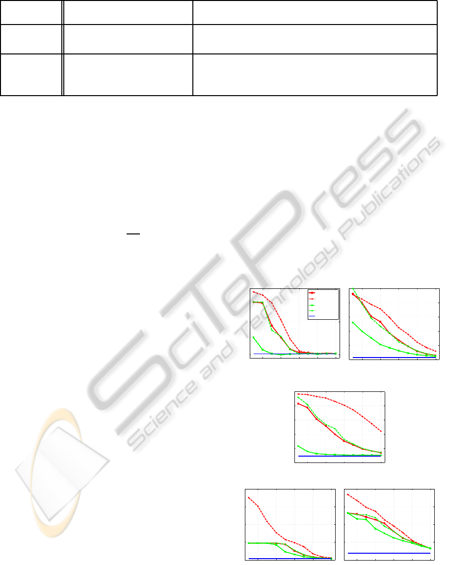
Table 1: Loss functions and their corresponding subgradients for classiﬁcation and regression tasks.

Task Loss Function, ℓ Subgradient Estimate, G



j−1



;ξ



Classiﬁcation max{1−y(w

φ(t) + b), 0}



λγ

j−1

+ d



, d

(

−y

if y

j−1

+ b

j−1

) < 1

0 otherwise

Regression max{|y −(w

φ(t) + b)|−ε,0}



λγ

j−1

+ d



, d











−1 if y

> V

j−1

+ b

j−1

+ ε,

1 if y

< V

j−1

+ b

j−1

−ε,

0 otherwise.

When we omit the intercept b in (PL), f(x) be-

comes strongly convex. We can then use steplength

= 1/(λj), and omit the averaging, to achieve faster

convergence in theory. We refer to the resulting algo-

rithm after modiﬁcation as ASSET

∗

. When λ ≈ 0,

convergence of ASSET

∗

can be quite slow unless we

have D

≈ 0 as well.

Theorem 2. Given the output x

and f(x

∗

), ASSET

∗

with η

= 1/(λ j) satisﬁes

E[ f(x

) − f(x

∗

)] ≤ max

(





, D

)

/N.

4 COMPUTATIONAL RESULTS

We implemented Algorithm 1 based on the open-

source Pegasos code (ours is available at

http://

pages.cs.wisc.edu/

sklee/asset/

.) The ver-

sions of our algorithms that use kernel matrix approx-

imation are referred to as ASSET

and ASSET

∗

while those with feature mapping approximation are

called ASSET

and ASSET

∗

. For direct comparisons

with other codes, we do not include intercept terms,

since some of the other codes do not allow such terms

to be used without penalization. All experiments with

randomness are repeated 50 times.

Table 2 summarizes the six binary classiﬁca-

tion tasks we use, indicating the values of param-

eters λ and σ selected using SVM-Light to maxi-

mize the classiﬁcation accuracy on each validation

set. (For

MNIST-E

, we use the same parameters as

MNIST

.) For the ﬁrst ﬁve moderate-size tasks, we

compare all of our algorithms against four publicly

available codes: two cutting-plane methods CPNY

and CPSP, and the other two are SVM-Light and

LASVM. The original SVM-Perf (Joachims, 2006)

and OCAS (Franc and Sonnenburg, 2008) are not in-

cluded because they cannot handle nonlinear kernels.

For

MNIST-E

, we compare our algorithms using fea-

ture mapping approximation to LASVM.

For our algorithms, the averaging parameter is set

N = m −100 for all cases (averaging is performed

for the ﬁnal 100 iterates). The test error values are

computed using the efﬁcient schemes of Section 2.4.

4.1 Effect of Approximation Dimension

To investigate the effect of kernel approximation di-

mension on prediction accuracy, we vary the dimen-

sion parameter s in Section 2.3 in the range [2, 1024],

with the eigenvalue threshold ε

= 10

−16

. Note that s

is an upper bound on the actual approximation dimen-

sion d for ASSET

, but is equal to d for ASSET

The codes CPSP and CPNY have a parameter similar

to s (as an upper bound of d). For purposes of com-

parison, we set that parameter to s. For the ﬁrst ﬁve

2 4 6 8 10

0.15

0.2

0.25

log

(s)

Test error rate

ASSET

CPSP

CPNY

SVM−Light

(a) ADULT.

2 4 6 8 10

0.1

0.2

0.3

0.4

0.5

(b) MNIST.

2 4 6 8 10

0.1

0.2

0.3

0.4

0.5

2 4 6 8 10

0.1

0.2

0.3

0.4

(d) IJCNN.

2 4 6 8 10

0.1

0.2

0.3

0.4

0.5

(e) COVTYPE.

Figure 1: The effect of the approximation dimension to the

test error. The x-axis shows the values of s in log scale.

ICPRAM 2012 - International Conference on Pattern Recognition Applications and Methods

226

Table 2: Data sets and training parameters.

http://www.csie.ntu.edu.tw/∼cjlin/libsvmtools/datasets/,

http://leon.bottou.org/

papers/loosli-canu-bottou-2006/.

Name m (train) valid/test n (density) λ σ Note

ADULT

32561 8140/8141 123 (11.2%) 3.07e-08 0.001 UCI Repository.

MNIST

58100 5950/5950 784 (19.1%) 1.72e-07 0.01 Digits 0-4 vs. 5-9.

CCAT

78127 11575/11574 47237 (1.6%) 1.28e-06 1.0 RCV1-v2 collection.

IJCNN

113352 14170/14169 22 (56.5%) 8.82e-08 1.0 IJCNN 2001 Challenge

COVTYPE

464809 58102/58101 54 (21.7%) 7.17e-07 1.0 Forest cover type 1 vs. rest.

MNIST-E

1000000 20000/20000 784 (25.6%) 1.00e-08 0.01 An extended MNIST set

Table 3: Training CPU time (in seconds, h:hours) and test error rate (%) in parentheses. Kernel approximation dimension is

varied by setting s = 512 and s = 1024 for ASSET

, ASSET

∗

, CPSP and CPNY. Decomposition methods do not depend on

s, so their results are the same in both tables.

Subgradient Methods Cutting-plane Decomposition

s = 512 ASSET

ASSET

∗

CPSP CPNY LASVM SVM-Light

ADULT

23(15.1±0.06) 24(15.1±0.06) 3020(15.2) 8.2h(15.1) 1011(18.0) 857(15.1)

MNIST

97 (4.0±0.05) 101 (4.0±0.04) 550 (2.7) 348 (4.1) 588 (1.4) 1323 (1.2)

CCAT

95 (8.2±0.08) 99 (8.3±0.06) 800 (5.2) 62 (8.3) 2616 (4.7) 3423 (4.7)

IJCNN

87 (1.1±0.02) 89 (1.1±0.02) 727 (0.8) 320 (1.1) 288 (0.8) 1331 (0.7)

COVTYPE

697(18.2± 0.06) 586(18.2±0.07) 1.8h(17.7) 1842(18.2) 38.3h(13.5) 52.7h(13.8)

s = 1024 ASSET

ASSET

∗

CPSP CPNY LASVM SVM-Light

ADULT

78(15.1±0.05) 83(15.1±0.04) 3399(15.2) 7.5h(15.2) 1011(18.0) 857(15.1)

MNIST

275 (2.7±0.03) 275 (2.7±0.02) 1273 (2.0) 515 (2.7) 588 (1.4) 1323 (1.2)

CCAT

265 (7.1±0.05) 278 (7.1±0.04) 2950 (5.2) 123 (7.2) 2616 (4.7) 3423 (4.7)

IJCNN

307 (0.8±0.02) 297 (0.8±0.01) 1649 (0.8) 598 (0.8) 288 (0.8) 1331 (0.7)

COVTYPE

2259(16.5±0.04) 2064(16.5±0.06) 4.1h(16.6) 3598(16.5) 38.3h(13.5) 52.7h(13.8)

moderate-size tasks, we ran our algorithms for 1000

epochs (1000m iterations). The baseline performance

values were obtained by SVM-Light.

Figure 1 shows the results. Since ASSET

and

ASSET

∗

yield very similar results in all experiments,

we do not plot ASSET

∗

. (For the same reason we

show ASSET

but not ASSET

∗

.) For small σ values,

as in Figure 1(a), all codes achieve good classiﬁca-

tion performance with small dimension. In other data

sets, the chosen values of σ are larger and the intrin-

sic rank of the kernel matrix is higher, so performance

continues to improve as s increases.

CPSP generally requires lower dimension than the

others to achieve the same prediction performance.

CPSP spends extra time to construct optimal ba-

sis functions, whereas the other methods depend on

random sampling. However, all approximate-kernel

methods including CPSP suffer considerably from the

restriction in dimension for

COVTYPE

4.2 Speed Comparison

Here we ran all algorithms other than ours with their

default stopping criteria. For ASSET

and ASSET

∗

we checked the classiﬁcation error on the test sets ten

times per epoch, terminating when the error matched

the performance of CPNY. (Since this code uses a

similar Nystr¨om approximation of kernel, it is the one

most directly comparable with ours in terms of classi-

ﬁcation accuracy.) The test error was measured using

the iterate averaged over the 100 iterations immedi-

ately preceding each checkpoint.

Results are shown in Table 3 for s = 512 and

s = 1024. (LASVM and SVM-Light do not depend

on s and so their results are the same in both tables.)

Our methods are the fastest in most cases. Although

the best classiﬁcation errors among the approximate

codes are obtained by CPSP, the runtimes of CPSP

are considerably longer than for our methods. In

fact, if we compare the performance of ASSET

with

s = 1024 and CPSP with s = 512, ASSET

achieves

similar test accuracy to CPSP (except for

CCAT

) but is

faster by a factor between two and forty.

It is noteworthy that ASSET

shows similar per-

formance to ASSET

∗

despite the less impressive the-

oretical convergence rate of the former. This is be-

cause the values of optimal parameter λ were near

zero, and thus the objective function lost the strong

convexity condition required for ASSET

∗

to work.

We observed similar slowdown of Pegasos and SGD

ASSET: APPROXIMATE STOCHASTIC SUBGRADIENT ESTIMATION TRAINING FOR SUPPORT VECTOR

MACHINES

227

0 1 2 3 4 5 6 7

0.1

0.2

0.3

0.4

0.5

Time (h)

Test error

d=1024

ASSET

ASSET*

0 1 2 3 4 5 6 7

0.1

0.2

0.3

0.4

0.5

Time (h)

Test error

d=4096

0 1 2 3 4 5 6 7

0.1

0.2

0.3

0.4

0.5

Time (h)

Test error

d=16384

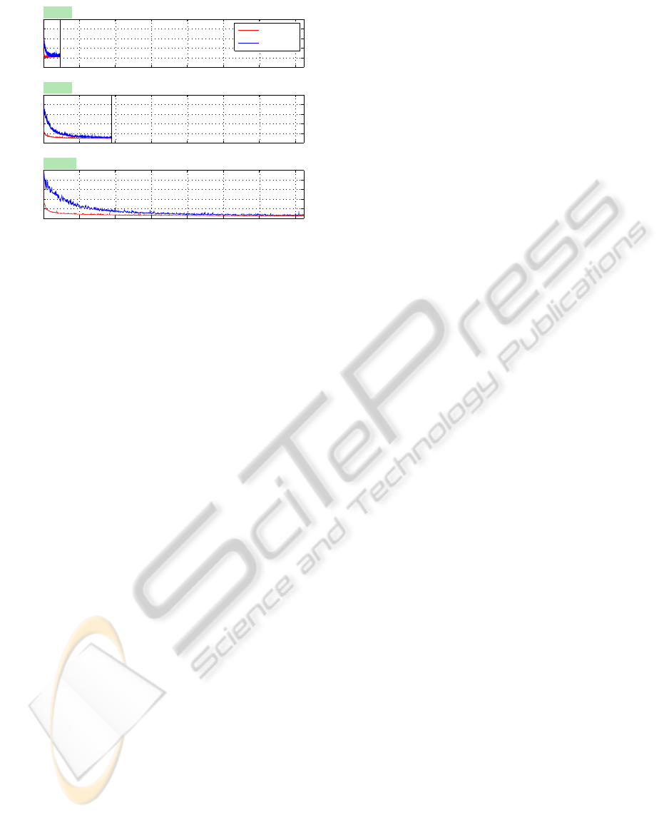
Figure 2: Progress of ASSET

and ASSET

∗

to their com-

pletion (

MNIST-E

), in terms of test error rate.

when λ approaches zero for linear SVMs.

4.3 Large-scale Performance

We take the ﬁnal data set

MNIST-E

and compare the

performance of ASSET

and ASSET

∗

to the online

SVM code LASVM. For a fair comparison, we fed the

training samples to the algorithms in the same order.

Figure 2 shows the progress on a single run of

our algorithms, with various approximation dimen-

sions d (which is equal to s in this case) in the range

[1024, 16384]. Vertical bars in the graphs indicate

the completion of training. ASSET

tends to con-

verge faster and shows smaller test error values than

ASSET

∗

, despite the theoretical slower convergence

rate of the former. With d = 16384, ASSET

and

ASSET

∗

required 7.2 hours to ﬁnish with a solu-

tion of 2.7% and 3.5% test error rate, respectively.

LASVM produced a better solution with only 0.2%

test error rate, but it required 4.3 days of computation

to complete a single pass through the same data.

5 CONCLUSIONS

We haveproposed a stochastic gradient framework for

training large-scale and online SVMs using efﬁcient

approximations to nonlinear kernels, which can be ex-

tended easily to other kernel-based learning problems.

ACKNOWLEDGEMENTS

The authors acknowledge the support of NSF Grants

DMS-0914524 and DMS-0906818. Part of this work

has been supported by the German Research Founda-

tion (DFS) grant for the Collaborative Research Cen-

ter SFB 876: “Providing Information by Resource-

Constrained Data Analysis”.

REFERENCES

Bordes, A., Ertekin, S., Weston, J., and Bottou, L. (2005).

Fast kernel classiﬁers with online and active learning.

Journal of Machine Learning Research, 6:1579–1619.

Bottou, L. (2005). SGD: Stochastic gradient descent.

http://leon.bottou.org/projects/sgd.

Chapelle, O. (2007). Training a support vector machine in

the primal. Neural Computation, 19:1155–1178.

Drineas, P. and Mahoney, M. W. (2005). On the nystrom

method for approximating a gram matrix for improved

kernel-based learning. Journal of Machine Learning

Research, 6:2153–2175.

Franc, V. and Sonnenburg, S. (2008). Optimized cutting

plane algorithm for support vector machines. In Pro-

ceedings of the 25th International Conference on Ma-

chine Learning, pages 320–327.

Joachims, T. (1999). Making large-scale support vector ma-

chine learning practical. In Advances in Kernel Meth-

ods - Support Vector Learning, pages 169–184. MIT

Press.

Joachims, T. (2006). Training linear SVMs in linear time.

In International Conference On Knowledge Discovery

and Data Mining, pages 217–226.

Joachims, T., Finley, T., and Yu, C.-N. (2009). Cutting-

plane training of structural svms. Machine Learning,

77(1):27–59.

Joachims, T. and Yu, C.-N. J. (2009). Sparse kernel svms

via cutting-plane training. Machine Learning, 76(2-

3):179–193.

Lee, S. and Wright, S. J. (2011). Approximate stochastic

subgradient estimation training for support vector ma-

chines. http://arxiv.org/abs/1111.0432.

Nemirovski, A., Juditsky, A., Lan, G., and Shapiro, A.

(2009). Robust stochastic approximation approach to

stochastic programming. SIAM Journal on Optimiza-

tion, 19(4):1574–1609.

Nemirovski, A. and Yudin, D. B. (1983). Problem complex-

ity and method efﬁciency in optimization. John Wiley.

Rahimi, A. and Recht, B. (2008). Random features for

large-scale kernel machines. In Advances in Neu-

ral Information Processing Systems 20, pages 1177–

1184. MIT Press.

Shalev-Shwartz, S., Singer, Y., and Srebro, N. (2007). Pe-

gasos: Primal estimated sub-gradient solver for svm.

In Proceedings of the 24th International Conference

on Machine Learning, pages 807–814.

Shalev-Shwartz, S., Singer, Y., Srebro, N., and Cotter,

A. (2011). Pegasos: Primal estimated sub-gradient

solver for svm. Mathematical Programming, Series

B, 127(1):3–30.

Zinkevich, M. (2003). Online convex programming and

generalized inﬁnitesimal gradient ascent. In Proceed-

ings of the 20th International Conference on Machine

Learning, pages 928–936.

ICPRAM 2012 - International Conference on Pattern Recognition Applications and Methods

228