
GRADIENT ARTEFACT CORRECTION IN THE EEG
SIGNAL RECORDED WITHIN THE fMRI SCANNER
José L. Ferreira
1
, Pierre J. M. Cluitmans
1
and Ronald M. Aarts
1,2
1
Department of Electrical Engineering, Eindhoven University of Technology, Eindhoven, The Netherlands
2
Philips Research Laboratories Eindhoven, Eindhoven, The Netherlands
Keywords: Combined EEG-fMRI, Imaging artefact correction, Average artefact subtraction, Artefact template
variability modelling.
Abstract: In recent years, combined EEG-fMRI has become a powerful brain imaging technique which is largely
employed in clinical and neuroscience research. Parallel to the achievements reached in this area, a number
of challenges remain to be overcome in order to consolidate such technique as an independent and effective
method for brain imaging. In particular, the occurrence of gradient artefacts in the EEG signal due to the
magnetic field of the fMRI magnetic scanner. This paper presents a proposal for modelling the variability of
the gradient artefact template which makes use of the standard deviation and the slope differentiator
between consecutive samples of the signals. Combination of such a model with the average artefact
subtraction method achieves a reasonable elimination of the gradient artefact from EEG recordings.
1 INTRODUCTION
Combined EEG-fMRI (acquisition of
electroencephalogram during functional magnetic
resonance imaging) is a technique for multimodal
brain activity mapping that has got a broad usage for
research and clinical purposes (Villringer et al.,
2010). Ritter and Villringer (2006) reinforce that co-
registered EEG-fMRI has attracted the interest of
several researchers and clinicians last years and it
has revealed itself a promising and additional
monitoring tool of the human brain activity.
Gonçalves et al. (2007) mention that although
such a brain imaging technique was first applied in
the field of epilepsy, nowadays it has been extended
to other types of neuroscience studies and
applications. Villringer et al. (2010) mention that
only simultaneous EEG-fMRI offers the opportunity
to relate both brain imaging modalities to actual
brain events, a characteristic which is relevant for
solving numerous research questions in basic and
cognitive neuroscience.
Parallel to the breakthroughs achieved by using
simultaneous combination of EEG-fMRI as an
independent brain imaging technique, some
problems related to its use remain to be solved in
order to consolidate and to enable broadening its
applications range. That is the case of the occurrence
of artefacts in the EEG signal caused by the
variation of the magnetic fields of the fMRI scanner,
the so-called “gradient” or “imaging acquisition”
artefact (Mulert and Hegerl, 2009).
2 OBJECTIVES
Gradient artefacts completely obscure the EEG, as
illustrated in figure 1. According to Ritter et al.
(2010), this type of artefact occurs in the EEG signal
due to the voltage induced by the application of
rapidly varying magnetic field gradients for spatial
encoding of the MR signal and radiofrequency
pulses (RF) for spin excitation in the circuit formed
by the electrodes, leads, patient and amplifier.
The waveform of the gradient artefact caused by
one RF pulse is approximately the differential
waveform of the corresponding RF pulse. Imaging
acquisition artefacts have amplitudes that can be
several orders of magnitude higher than the neuronal
EEG signal. Artefact amplitudes associated to the
gradient switching (10
3
to 10
4
μV) are generally
much larger than those arising from RF pulses (up to
10
2
μV) (Ritter et al., 2010).
110
Ferreira J., Cluitmans P. and Aarts R..
GRADIENT ARTEFACT CORRECTION IN THE EEG SIGNAL RECORDED WITHIN THE fMRI SCANNER.
DOI: 10.5220/0003788001100117
In Proceedings of the International Conference on Bio-inspired Systems and Signal Processing (BIOSIGNALS-2012), pages 110-117
ISBN: 978-989-8425-89-8
Copyright
c
2012 SCITEPRESS (Science and Technology Publications, Lda.)
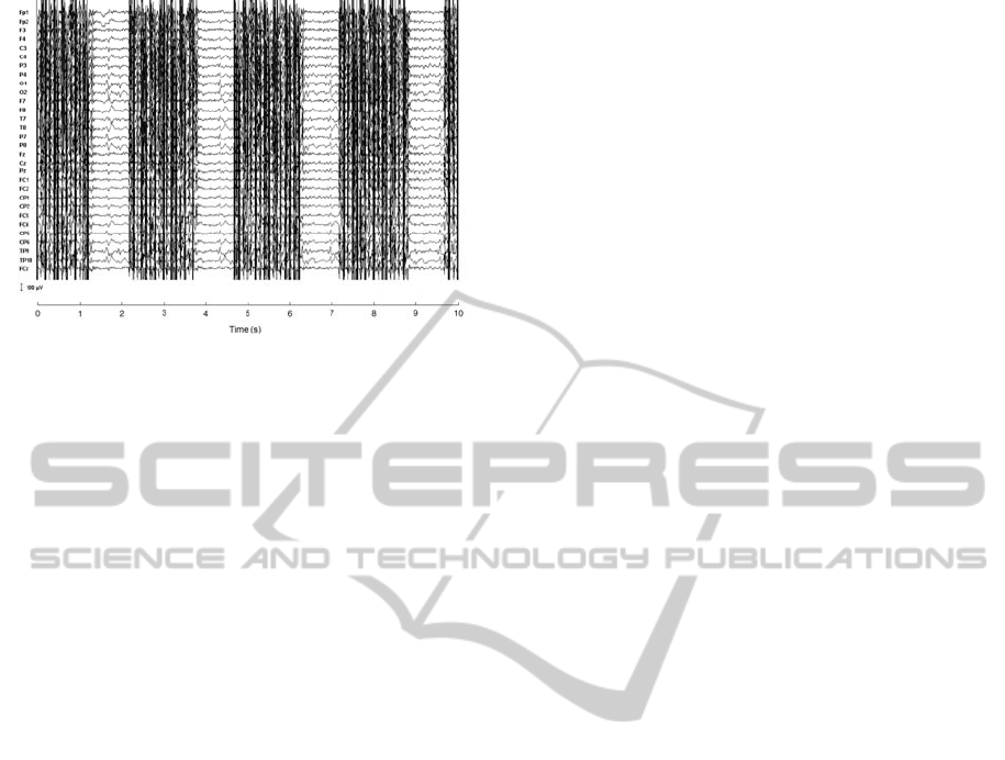
Figure 1: Imaging artefact in ongoing EEG data. Adapted
from Mantini et al. (2007).
As discussed by Ritter et al. (2010), the
frequency range of the gradient artefact exceeds that
of standard clinical EEG, nevertheless the EEG
recording is dominated by harmonics of the
repetitive slice convolved with harmonics in the
range of frequency of the volume repetitive
frequency. The frequency of these harmonics
overlaps the range frequency of the EEG signal.
Moreover, also as mentioned by Ritter et al., such
artefacts have a strong deterministic component
because the preprogrammed nature of RF and
gradient switching.
In literature, some techniques are suggested in
order to attempt minimizing the effects of gradient
artefacts in the EEG signal. For example, it is
possible to reduce their magnitude at the source by
laying out, immobilising and twisting the EEG leads,
using a bipolar electrode configuration and using a
head vacuum cushion. Further, depending on the
application, a periodic interleaved approach,
whereby the MR signal acquisition is suspended at
regular intervals, could be used as well (Ritter et al.,
2010).
Gonçalves et al. (2007) mention that concerning
continuous MR acquisition, dedicated software
solutions have to be developed in order to correct
gradient artefacts in the electroencephalogram.
Some post-processing signal methods for correction
of gradient artefacts in the EEG signal are based
upon time or frequency domain analysis which make
use of different mathematical and computational
digital signal processing approaches like spectrum
analysis, principal component analysis, independent
component analysis and average artefact subtraction
(Gonçalves et al., 2007).
According to Allen et al. (2000), the average
artefact subtraction methodology consists of the
calculation of an average imaging artefact waveform
or template over a fixed number of samples, and it is
then subtracted from the EEG signal for each
sample.
Performing average artefact subtraction alone
does not result to satisfactory quality of corrected
signal, demanding the need for further residuals
correction (Allen et al., 2000; Gonçalves et al.,
2007). These authors also propose the use of
adaptive noise cancelling for attenuating the
remaining residuals from the subtraction by using
low-pass filters, smoothing and downsampling.
However, according to Van de Velde et al. (1998),
the use of filtering could result in removing original
component frequencies of the EEG signal.
The objectives of the current paper are to present
an alternative approach for cleaning up such
residuals by employing a specific model for
evaluating and quantifying the variability of the
imaging artefact. The proposed methodology is
based upon information about the variance of the
averaged template artefact as well as on the slope
differentiator of the EEG signals under analysis.
3 MATERIALS AND METHODS
3.1 Features of the Data under
Analysis
Simultaneous EEG and fMRI data were collected for
a research focused on epilepsy and post-traumatic
stress disorder (PTSD), jointly developed by the
department of Psychiatry of Universiteit Medisch
Centrum Utrecht, the Research Centre Military
Mental Health Care in the Dutch Central Military
Hospital in Utrecht and the Department of Research
and Development of the Epilepsy Center of
Kempenhaeghe in Heeze (The Netherlands).
Data were recorded from patients characterized
as military veterans with PTSD which were in
mission abroad through the outpatient clinic of the
Military Mental Health Care. All participants were
male and aged between 18 and 60 years.
3.2 Protocol for EEG-fMRI Data
Collection
Functional magnetic resonance imaging scanning
was carried out using a 3 T Scanner (Philips,
Eindhoven, The Netherlands) at Kempenhaeghe
Epilepsy Center. An MRI-compatible 64 channel
polysomnograph was used to collect one ECG
channel, two EOG channels, one EMG and 60 EEG
GRADIENT ARTEFACT CORRECTION IN THE EEG SIGNAL RECORDED WITHIN THE fMRI SCANNER
111

channels. In the current work, the ECG signal was
used for synchronization purposes. EEG electrodes
positioning was in accordance with the international
10-20 system electrodes placement.
EEG-fMRI data were collected during 45
minutes, before the period that the patient should
sleep. After application of the EEG cap, the subjects
were scanned using a functional echo-planar
imaging sequence with 33 transversal slices
(thickness 3 mm, TE 30 ms, TR 2500 ms).
The used electroencephalogram device for
collecting the EEG signals possesses an appropriate
built-in notch filter. The sampling rate for signal
acquiring was 2048 Hz.
3.3 General Average Artefact
Subtraction Overview
The basic idea of the average subtraction approach
consists of estimating an average template of the
gradient artefact along an observed range of the
EEG signal, and then subtracting this template from
the electroencephalogram at those regions where the
artefact occurs (Allen et al., 2000). The average
artefact subtraction can be described by the
following expression:
s
iii,rawi,corct
EEGGEE
−
−= Γ
,
(1)
where i runs over the number of samples within the
entire EEG data set; i-i
s
is the time sample along the
selected EEG segments considered for average;
EÊG
corct
and EEG
raw
are respectively the corrected
and the uncorrected (raw) EEG signals; and Γ is the
template to be subtracted.
According to the methodology proposed by
Allen et al. (2000) to calculate such a template, the
EEG
raw
is divided in segments of fixed length (S
number of samples). The resulting averaging from
samples situated at the same segment position i-i
s
corresponds to the template epoch
s
ii−
Γ .
Allen et al. (2000) and Gonçalves et al. (2007)
also consider the need for interpolation and
extrapolation along the obtained fixed segment
length. According to the approach for average
gradient subtraction proposed by Gonçalves et al.
(2007), interpolation is necessary since in general
the clocks of the EEG and fMRI are uncalibrated
and, in consequence, misaligned. Thus, a small time
shift should be applied in order to compensate the
misalignment and to eliminate the variation of the
number of epochs among the slices segments.
Gonçalves et al. (2007) still take into account
estimation of some parameters which must be
computed before carrying out the artefact
subtraction like the slice time (ST) and the dead time
(DT) which are determined by minimizing a cost
function that is related to the ratio between EÊG
corct
and EEG
raw
.
3.4 Overview of the Average Artefact
Subtraction Methodology
Employed in this Work
In order to perform the estimation of the corrected
EEG, EÊG
corct
, the model described in (1) was
employed. In this sense, estimation of Γ was done
by dividing the chosen range of the observed
EEG
raw
in segments with fixed length, as proposed
by Allen et al. (2000) and Gonçalves et al. (2007).
However, due to some specific features observed in
the data analysed in the current work, a different
approach to estimate the length of those segments
was used.
Observation of the raw EEG data recorded
during the MR scanning revealed that the slice
length could be estimated by evaluation of the
distance between typical peaks noticed in the raw
EEG or ECG recordings that can be attributed to the
magnetic fields switching within the MR scanner
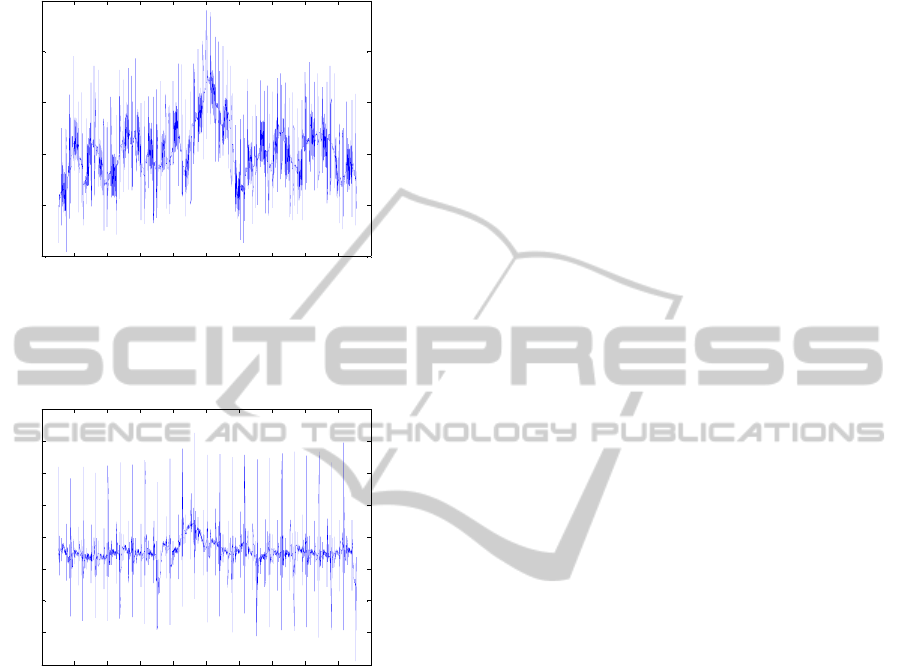
(Ritter et al., 2010). Figures 2 and 3 show the
occurrence of those peaks in 2 s-segments of the raw
EEG (electrode position F8) and raw ECG around
the time instant 429.4 s.
It is important to highlight that estimation of
such a distance from the EEG data recorded within
the scanner was necessary since: i) the
electromagnetic properties of different sources of
the system constituted by the electroencephalograph,
the fMRI scanner and patient have influence on the
artefact generation and morphology; ii) that is the
existing condition for the available data under
analysis. Thereby, it could not be evaluated just by
placing one electrode directly in the fMRI scanner.
Performing measurement of the distance
between peaks by using such a procedure allowed to
estimate the value of ST around (155 ± 1) epochs
that correspond to a time interval of approximately
(0.07568 ± 0.00050) s considering the data under
analysis in this work.
Thus, as a first approach, the used segment
length was the slice length itself, and EEG was
divided in segments of 155 epochs, according to the
measured distance between the peaks corresponding
to the beginning of each MR slice. In the case of the
segments that contained more or less than 155
epochs, extrapolation or interpolation were done in
order to fix the length of the segments and therefore
BIOSIGNALS 2012 - International Conference on Bio-inspired Systems and Signal Processing
112
to compensate the misalignment between the EEG
and fMRI clocks (Gonçalves et al., 2007).
428.4 428.6 428.8 429 429.2 429.4 429.6 429.8 430 430.2 430.4
2.55
2.555
2.56
2.565
2.57
2.575
x 10
4
Raw EEG signal - F8
Signal (
μ
V)
Time (s)
Figure 2: 2 s-segment around the time instant 429.4 s of
the raw EEG signal (electrode position F8), showing the
peaks caused by MR switching.
428.4 428.6 428.8 429 429.2 429.4 429.6 429.8 430 430.2 430.4
2.2
2.3
2.4
2.5
2.6
2.7
2.8
2.9
3
x 10
4
Raw ECG signal
Signal (
μ
V)
Time (s)
Figure 3: 2 s-segment around the time instant 429.4 s for
the raw ECG signal, showing the peaks caused by MR
switching.
The algorithm used for performing the average
subtraction was adapted from Bishop (2006) and
Press et al. (1992), and is based upon the idea that
the mean of a random variable corresponds to the
point where the random variable has the minimum
variance. By this approach, epochs from the
different segments in which the raw EEG was
divided and have a corresponding position within the
slice,
j,i,raw
EEG
, can be related to an initial choice
for the template average epoch at the same slice
position,
s
i-i
μ (=
s
ii−
Γ ), by the following cost
function:
∑
=
−=
J
1j
j,iraw,i-i
s
i-is
EEG
2
)μ()(μΨ
s
i-i
,
(2)
where J is the number of slices considered for
averaging. The rationale for using this formula is
that in addition to calculate the averaged gradient
artefact template, minimization of (2) provides to
estimate jointly the variance (standard deviation)
associated to each epoch, parameter which is used
during modelling and correction of the artefact
variability as described in the next section. (2) can
be rewritten into the following matrix format:
KK
T
⋅=)(μΨ
s
i-is
i-i
,
(3)
where K is a vector with Jx1 components
s
i-ij,iraw,j
EEGK μ−=
. Therefore, the value of
s
i-i
Ψ
is the variance associated to the template
epoch i-i
s
. Finally, the values of EÊG
corct
(and Γ)
can be calculated from:
T
K
K
Z
⋅
=
.
(4)
The square root of the diagonal elements of Z
corresponds to the values of EÊG
corct,i
.
3.5 Modelling of Imaging Artefact
Template Variability
For elimination of the remaining residuals in the
EÊG
corct
, a specific model is proposed for
attempting to quantify the artefact variability. The
use of this alternative approach was preferred since,
according to Van de Velde et al. (1998), the use of
filtering, as is done for conventional residuals
elimination, could also remove some original
frequencies of the EEG signal. Furthermore, the
remaining artefact residuals can be attributed to the
template variability.
Klados et al. (2009) suggest the use of an
adaptive method whereby it is possible to
approximate the EÊG
corct
to the true EEG.
According to that methodology, the template
variability is evaluated by multiplying each artefact
template sample by an estimated factor â
i
, and then
subtraction is processed as follows:
s
iiii,rawi,corct
aEEGGEE
−
−= Γ
.
(5)
The expression above is an adaptive extension of
(1) whose limit referred to the filter parameter â
i
allows refining the value of EÊG
corct
:
i,corcti,corct
aâ
EEGGEE
ii
=
→
lim
.
(6)
Therefore as far as the parameter â is approached
to the optimal value of the adaptive filter a, the value
of EÊG
corct
tends to the true EEG.
GRADIENT ARTEFACT CORRECTION IN THE EEG SIGNAL RECORDED WITHIN THE fMRI SCANNER
113

In the current work, this method was further
modified in such a way that â is changed to a new
non-filter parameter â’ and equations (5) and (6)
become:
iii,corcti,corct
R'aGEEEEG
−=
,
(7)
where the product of the corresponding elements of
the vectors â’ and R acts as an initial estimation of
the remaining residual in the EEG. Hence, (7) allows
to calculate a refinement for the value of the
corrected EEG by subtracting an estimation of the
remaining residual from the corresponding unrefined
value obtained for EÊG
corct
.
As the parameters â’ and R should represent the
variability of the gradient artefact, their estimation
took into account specific properties of the raw,
corrected signal and true EEG that are supposed to
reflect that variability. The standard deviation
associated to the averaged imaging artefact and the
signal slope differentiator were chosen as the
properties of the signals that represents the
variability, the former was associated to â’ and the
latter to R.
Concerning the standard deviation associated to
the averaged artefact, it is a natural choice since it is
a measurement of the variability of a random
variable around the mean (Papoulis and Pillai,
2002). According to the GUM (2008) the standard
deviation (or the variance) also could be seen as a
component of the uncertainty measurement
associated with the estimated average, and therefore
could be used for quantifying and correcting the lack
of information about the variability of the random
variable.
The choice of the slope differentiator is in
accordance with Van de Velde et al. (1998) that
describe such a signal parameter associated to the
large signal magnitudes as being particularly useful
for detection of the high-frequency properties of the
muscle artefact. At the same way, by observing the
EEG signals under analysis, it is noticed that high-
frequency as well as large signal magnitudes can be
attributed to the gradient artefact. Thereby, in our
work, the slope variation is also used to identify the
imaging acquisition artefact. Moreover, a new
approach is proposed to quantify the variability
making use of the signal slope as well, as described
below.
In our approach, estimation of the parameter R is
based upon the simple differentiation of EEG
raw
,
diff (EEG
raw
), EÊG
corct
, diff (EÊG
corct
), and the
artefact free EEG. An artefact free EEG interval
could be obtained from the available data, from
approximately the first 5 s of the recordings of each
EEG channel, allowing estimating the corresponding
values for the slope differentiator.
By analysing the artefact free interval, it could
be observed that the maximum value of the slope
differentiator of the true EEG is estimated around
15 μV/sample. The values observed for the same
parameter, considering EEG
raw
and EÊG
corct
, are
usually much higher when compared to the true
EEG in such a way that it allows identification of
epochs as being artefact free or not, which is in
accordance with the methodology proposed by Van
de Velde et al. (1998). The values of the elements of
R were quantified by taking into account the
normalized values of diff (EÊG
corct
), whose
maximum value was considered as being equal to 1,
as follows:
)(max
)(
corct
GEE
diff
GEEGEE
R
i,corct1i,corct
i,norm
−
=
+
.
(8)
Thus, R
norm,i
corresponds to the normalized value
of diff (EÊG
corct
).
As mentioned above, the elements of vector â’
(i.e., â
i
’) were related to the value of standard
deviation
s
ii
s
−
of the gradient average artefact, as
indicated in (9) and 10:
s
iii
s'a
ˆ
−
=
;
(9)
s
ii
s
−
is equal to the root square of the template
variance:
ss
-iiii
s Ψ=
−
.
(10)
Finally, considering (8), (9) and (10), expression
(7) can be rewritten as:
i,normiii,corcti,corct
RsGEEEEG
s
−
−=
.
(11)
Therefore, the limit described in equation (6) is
carried out by performing the subtraction indicated
in (11) iteratively, until a predetermined threshold
value is reached. In this work, the threshold was set
as being the value of diff (EEG
corct
) coincident with
the mean plus the standard deviation calculated for
the slope differentiator of the true EEG (estimated
around 1.5 μV/sample for the available data).
It is worthwhile to consider that in our approach
the values of the parameter R
norm,i
act as weights
varying from 0 to 1 which indicate what percentage
of the standard deviation should be applied for
refinement of EÊG
corct
,
i
. In other words, the value of
R
norm,i
acts as an indicator of the presence of the
gradient artefact in
EÊG
corct
(Van de Velde et al.,
1998) and at the same time indicates the amount of
correctness based on that should be applied on
EÊG
corct,i
.
s
ii
s
−
s
ii
s
−
BIOSIGNALS 2012 - International Conference on Bio-inspired Systems and Signal Processing
114
4 RESULTS
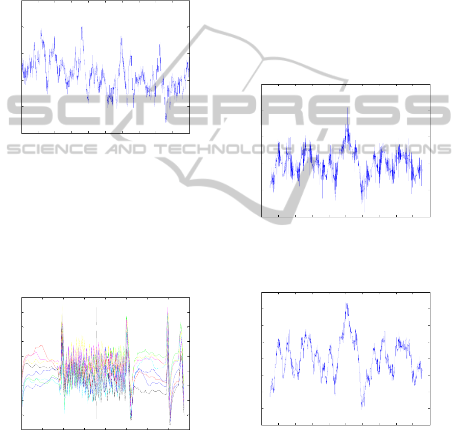
In figure 4, the artefact free 5 s-period of the raw
EEG corresponding to the EEG at channel F8 is
depicted. It is noticed that there is a DC offset in the
signal around 2.55 x 10
4
μV. A similar DC
component is also observed for the other electrode
EEG positions and ECG recording.
0 0.5 1 1.5 2 2.5 3 3.5 4 4.5 5
2.54
2.545
2.55
2.555
2.56
2.565
x 10
4
Raw EEG signal - F8
Signal (
μ
V)
Time (s)
Figure 4: Artefact free period of raw EEG signal
recording, corresponding to electrode position F8. A DC
component around 2.55 x 10
4
μV can be observed.
In order to estimate the artefact template Γ, a set
of eight subsequent segments (J = 8 slices) were
considered from the raw EEG signal. Figure 5 shows
one set of slices picked up from the raw EEG signal
already containing interpolated or extrapolated
epochs depending on the need, and used during the
calculations.
0 20 40 60 80 100 120 140 160
2.552
2.554
2.556
2.558
2.56
2.562
2.564
2.566
2.568
2.57
x 10
4
Γ
Epoch
Signal (
μ
V)
Set of eight slices considered for artefact template estimation
i-i
s
Figure 5: Set of eight (J = 8) subsequent EEG segments
slice-length (155 epochs) around the time instant of 430 s
considered for averaging. The average template Γ is
calculated considering corresponding epochs of each
segment (Allen et al., 2000).
Figure 6 shows the results of the average artefact
subtraction described by application of equations
(2), (3) and (4) on the raw EEG signal showed in
figure 2. Nevertheless the observed DC component
has been removed, in comparison to the artefact free
EEG signal of figure 4, a considerable amount of
remaining residual peaks uniformly distributed along
the signal resulting from the gradient artefact are
still observed in figure 6.
Hence, in order to obtain a better correction for
EÊG
corct
, equations (8) to (11) are then applied to
the signal of figure 6, resulting to the signal depicted
in figure 7. From this figure, it could be seen that the
noticed residuals in figure 6 were strongly cleaned
up.
428.4 428.6 428.8 429 429.2 429.4 429.6 429.8 430 430.2 430.4
-100
-50
0
50
100
150
Corrected EEG with remaining residuals - F8
Signal (
μ
V)
Time (s)
Figure 6: Signal resulting (EÊG
corct
) from application of
equations (2), (3) and (4) on the signal of figure 2.
428.4 428.6 428.8 429 429.2 429.4 429.6 429.8 430 430.2 430.4
-80
-60
-40
-20
0
20
40
60
80
Corrected EEG cleaned from residuals - F8
Signal (
μ
V)
Time (s)
Figure 7: Signal resulting (EEG
corct
) from application of
equations (8) to (11) on the signal of figure 6.
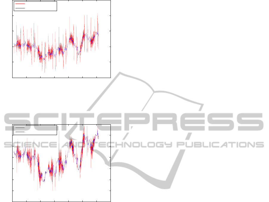
Finally, figures 8 and 9 depict zooming in (0.7 s-
segment length) around the time instant 430 s,
showing superposition of the signals raw EEG and
EEG
corct
, and the signals EÊG
corct
and EEG
corct
.
GRADIENT ARTEFACT CORRECTION IN THE EEG SIGNAL RECORDED WITHIN THE fMRI SCANNER
115
430 430.1 430.2 430.3 430.4 430.5 430.6 430.7
-100
-50
0
50
100
150
Raw EEG and EEG cleaned from residuals - F8
Signal (
μ
V)
Time
(
s
)
Raw EEG
Cleaned from residuals
Figure 8: 0.7 s-segment around the time instant 430 s of
the signal EEG
corct
(cleaned from residuals) superimposed
to the raw EEG (without DC offset).
430 430.1 430.2 430.3 430.4 430.5 430.6 430.7
-80
-60
-40
-20
0
20
40
60
EEG average subtracted and EEG cleaned from residuals - F8
Signal (
μ
V)
Time (s)
Average subtracted
Cleaned from residuals
Figure 9: 0.7 s-segment around the time instant 430 s of
the signal EEG
corct
(cleaned from residuals) superimposed
to EÊG
corct
(average subtracted).
5 DISCUSSION
As can be regarded in figure 8 and 9, combination of
the methods average artefact subtraction with the
approach here proposed for cleaning up the resulting
residuals from that subtraction have achieved a
strong elimination of the gradient artefact from the
raw EEG signal.
As regarded in figure 6, just the average artefact
subtraction approach described in equations (2), (3)
and (4) does not result to satisfactory elimination of
the artefact from the EEG signal since a
considerable amount of residuals remains in the
resulting corrected signal (figure 6). Such residuals
can be attributed to the variability of the imaging
artefact and this information is not taken into
account when only the average is used in the
correction. Nevertheless the waveform of the
gradient artefact possesses a strong deterministic
(Ritter et al., 2010) and reproducible component, as
could be noticed in figure 5, the variability
associated with the artefact provokes the presence of
residuals in the corrected EEG and, therefore, the
need for further correction.
Hence, in our approach for removing the artefact
residuals, it is proposed to use additional
characteristics from the available data which could
contain some information about the template
variability as well as which could enable to quantify
the magnitude of the residuals. The two chosen
signal characteristics were the standard deviation
associated to the averaged (Papoulis and Pillai,
2002; GUM, 2008) template and the signal slope
differentiator (Van de Velde et al., 1998), and
showed themselves fit those requirements since the
use of equations (5) to (11) allows elimination of the
residuals as is depicted in figure 7.
Therefore, combination of the average artefact
subtraction method and the methodology for
quantifying the variability of the template of the
imaging artefact proposed here reveals itself to be an
alternative method for cleaning up the EEG signal
from the gradient artefact, which could produce a
good quality for the resulting corrected signal.
Nevertheless the model described in equations (5) to
(11) constitutes a prototype and requires more
accurate refinement and validation, some advantages
of its application could be mentioned in comparison
to other methods.
Firstly, the employed approach is implemented
only in the time domain. In addition, it does not
requires insertion of markers in the EEG signal since
the value of important events associated to the MR
scanning like ST, DT and TR could be evaluated
directly from data (observed peaks in the raw signals
caused by the imaging artefact). Furthermore, the
entire estimation of the model parameters is based
upon the use of simple statistical parameters of the
signals like mean, standard deviation and mode.
Another observed advantage of the employed
methodology is that, in principle, a low number of
slices could be used during template averaging
without the need for using the slices of the entire
MR volume as well as recordings from other EEG
channels. This consideration could be useful in
future developments concerning real time
applications. Finally, in principle there is no need for
using filtering; this fact will be evaluated in future
steps for method validation.
The use of the synchronized ECG signal was
useful during application of the proposed
BIOSIGNALS 2012 - International Conference on Bio-inspired Systems and Signal Processing
116

methodology since the events related to the MR
scanning occur simultaneously in the EEG and the
ECG recordings, in such a way that the
electrocardiogram can be used for estimation of
relevant parameters associated to the proposed
correction methodology which also are valid for the
electroencephalogram.
6 CONCLUSIONS
A prototype model for quantifying the gradient
template variability combined with the average
artefact template subtraction methodology was
applied for removing gradient artefact from EEG
signals, and proves to be promising as an alternative
approach for obtaining a good signal correction.
As described in literature (Allen et al., 2000;
Gonçalves et al., 2007), the average artefact
subtraction alone does not result to satisfactory
quality of corrected signal, demanding the need for
further residuals correction. As discussed by Van de
Velde et al. (1998), the use of filtering could result
in removing original component frequencies of the
EEG signal. Therefore, in this work a model for
identification and quantification of the residuals to
be subtracted is proposed, instead the usual
employment of low-pass filtering for cleaning up the
remaining residuals.
In future work, the influence of a higher number
of slices (for instance, the entire number of slices of
the MR volume) must be checked as well as signal
estimation of the time intervals corresponding to the
dead time (DT) have to be carried out using the
presented approach. Also, the proposed model has to
be applied to a larger set of EEG clinical data in
order to evaluate its consistency.
Finally, as an additional recommendation for
future work, it should be analyzed if the proposed
methodology could be extended for correction of
other types of artefact as well as could be
consolidated as an alternative average subtraction
approach for signal correction.
ACKNOWLEDGEMENTS
We are grateful to Saskia van Liempt, M.D., and
Col. Eric Vermetten, M.D., Ph.D. from the
University Medical Center/Central Military
Hospital, Utrecht, for providing the data presented in
this work. This work has been made possible by a
grant from the European Union and Erasmus
Mundus – EBW II Project.
REFERENCES
Allen, P., Josephs, O., Turner, R., 2000. A method for
removing imaging artefact from continuous EEG
recorded during functional MRI. NeuroImage. 12.
Elsevier: 230-239.
Bishop, C., 2006. Pattern recognition and machine
learning. Springer: New York.
Gonçalves, S., Pouwels, P., Kuijer, J., Heethaar, R., de
Munck, J., 2007. Artefact removal in co-registered
EEG/fMRI by selective average subtraction. Clinical
Neurophysiology. 118. Elsevier: 823-838.
GUM, 2008. Evaluation of measurement data – Guide to
the expression of uncertainty in measurement. 1
st
ed.
JCGM.
Klados, M., Papadelis, C., Bamidis, P., 2009. A new
hybrid method for EOG artefact rejection. 9
th
International Conference on Information Technology
and Application in Biomedicine, ITAB 2009, Larnaca,
Cyprus, November 5-7, 2009, Proceedings: 4937-
4940.
Mantini, D., Perucci, M., Cugini, S., Romani, G., Del
Gratta, C., 2007. Complete artefact removal for EEG
recorded during continuous fMRI using independent
component analysis. NeuroImage. 34. Elsevier: 598-
607.
Mulert, C., Hegerl, U., 2009. Integration of EEG and
fMRI. In E. Kraft, G. Gulyás, E. Pöppel (eds.), Neural
correlation of thinking. Springer: Verlag, Berlin,
Heidelberg.
Papoulis, A.; Pillai, S., 2002. Probability, random
variables, and stochastic processes. 4
th
ed. New York:
McGraw-Hill.
Press, W.; Teukolsky, S.; Vetterling, W; Flannery, B.,
1992. Numerical recipes in C: the art of scientific
computing. 2
nd
ed. Cambridge University Press:
Cambridge.
Ritter, P., Becker, R., Freyer, F., Villringer, A., 2010. EEG
quality: the image acquisition artefact. In C. Mulert, L.
Limieux (eds.), EEG-fMRI: Physiological basis,
technique and applications. Springer: Verlag, Berlin,
Heidelberg.
Ritter, P., Villringer, A., 2006. Simultaneous EEG-fMRI.
Neuroscience and Biobehavioral Reviews. 30.
Elsevier: 823-838.
Van de Velde, R., Van Erp, G., Cluitmans, P., 1998.
Detection of muscle artefact removal in the normal
human awake EEG. Electroencephalography and
Clinical Neurophysiology. 107. Elsevier: 149-158.
Villringer, A., Mulert, C., Lemieux, L., 2010. Principles of
multimodal functional imaging and data integration. In
C. Mulert, L. Limieux (eds.), EEG-fMRI:
Physiological basis, technique and applications.
Springer: Verlag, Berlin, Heidelberg.
GRADIENT ARTEFACT CORRECTION IN THE EEG SIGNAL RECORDED WITHIN THE fMRI SCANNER
117
