
A DYNAMIC WRAPPER METHOD FOR FEATURE
DISCRETIZATION AND SELECTION
Artur Ferreira
1,3
and Mario Figueiredo
2,3
1
Instituto Superior de Engenharia de Lisboa, Lisboa, Portugal
2
Instituto Superior T´ecnico, Lisboa, Portugal
3
Instituto de Telecomunicac¸˜oes, Lisboa, Portugal
Keywords:
Feature discretization, Feature selection, Static discretization, Dynamic discretization, Wrapper approach,
Linde-Buzo-Gray algorithm.
Abstract:
In many learning problems, an adequate (sometimes discrete) representation of the data is necessary. For in-
stance, for large number of features and small number of instances, learning algorithms may be confronted
with the curse of dimensionality, and need to address it in order to be effective. Feature selection and fea-
ture discretization techniques have been used to achieve adequate representations of the data, by selecting an
adequate subset of features with a convenient representation. In this paper, we propose static and dynamic
methods for feature discretization. The static method is unsupervised and the dynamic method uses a wrapper
approach with a quantizer and a classifier, and it can be coupled with any static (unsupervised or supervised)
discretization procedure. The proposed methods attain efficient representations that are suitable for learning
problems. Moreover, using well-known feature selection methods with the features discretized by our methods
leads to better accuracy than with the features discretized by other methods or even with the original features.
1 INTRODUCTION
Datasets with large numbers of features and (rela-
tively) smaller numbers of instances are challenging
for machine learning methods. In fact, it is often the
case that many features are irrelevant or redundant for
the task at hand (e.g., learning a classifier) (Yu et al.,
2004; Peng et al., 2005); this may be specially harm-
ful with relatively small training sets, where these ir-
relevancies/redundancies are harder to detect.
To deal with such datasets, feature selection (FS)
and feature discretization (FD) methods have been
proposed to obtain data representations that are more
adequate for learning. FD aims at finding a represen-
tation of each feature that contains enough informa-
tion for the learning task at hand, while ignoring mi-
nor (possibly irrelevant) fluctuations. FS aims at re-
ducing the number of features, thus directly targeting
the curse of dimensionality problem, often allowing
the learning algorithms to obtain classifiers with bet-
ter performance. A byproduct of FD and FS is a re-
duction of the memory required to represent the data.
Both FD and FS are topics with a long re-
search history and a vast literature; regarding FD, see
(Dougherty et al., 1995), (Liu et al., 2002), (Witten
and Frank, 2005) for extensivereviews of many meth-
ods; regarding FS, see (Guyon et al., 2006), (Hastie
et al., 2009), and (Escolano et al., 2009) for compre-
hensive coverage and pointers to the literature.
1.1 Our Contribution
In this paper, we propose an unsupervised method for
static FD and a new method for dynamic FD. The dy-
namic discretization method uses a wrapper approach
with a quantizer and a classifier, and can be cou-
pled with any static (unsupervised or supervised) dis-
cretization procedure. The dynamic method assesses
the performance of each feature as discretization is
carried out; if it is found that the original representa-
tion is preferable to the discretized one, the original
feature is kept.
The remaining text is organized as follows. Sec-
tion 2 reviews supervised and unsupervised FD and
FS techniques. Section 3 presents the proposed static
and dynamic methods for FD. Section 4 reports the
experimental evaluation of our methods in compari-
son with other techniques. Finally, Section 5 ends the
paper with some concluding remarks and directions
for future work.
103
Ferreira A. and Figueiredo M. (2012).
A DYNAMIC WRAPPER METHOD FOR FEATURE DISCRETIZATION AND SELECTION.
In Proceedings of the 1st International Conference on Pattern Recognition Applications and Methods, pages 103-112
DOI: 10.5220/0003788201030112
Copyright
c
SciTePress

2 BACKGROUND
This section briefly reviews some of the most com-
mon unsupervised and supervised FD and FS tech-
niques that have proven effective for many learning
problems. This description is hugely far from be-
ing exhaustive, as FD and FS are two fields with
a long research history. The interested reader is
referred to the works of (Dougherty et al., 1995),
(Kotsiantis and Kanellopoulos, 2006), (Liu et al.,
2002), and (Witten and Frank, 2005), for re-
views of FD methods. Reviews of FS methods
were done by (Guyon and Elisseeff, 2003), (Guyon
et al., 2006), (Hastie et al., 2009), and (Escolano
et al., 2009); see also the following special issue:
jmlr.csail.mit.edu/papers/special/feature03.html.
2.1 Feature Discretization
FD can be performed in supervised or unsupervised
modes, i.e., using or not the class labels, and aims at
reducing the amount of memory as well as improv-
ing classification accuracy (Witten and Frank, 2005).
The supervised mode may lead, in principle, to better
classifiers. In the context of unsupervised scalar FD
(Witten and Frank, 2005), two efficient techniques are
commonly used:
. equal-interval binning (EIB), i.e., uniform quan-
tization with a given number of bits per feature;
. equal-frequency binning (EFB), i.e., non-uniform
quantization yielding intervals such that, for each
feature, the number of occurrences in each inter-
val is the same, leading to a uniform (i.e., maxi-
mum entropy) distribution; this technique is also
known as maximum entropy quantization.
In EIB, the range of values is divided into bins
of equal width. It is simple and easy to implement,
but it is very sensitive to outliers, thus may lead to
inadequate discrete representations. The EFB method
is less sensitive to outliers. The quantization intervals
have smaller width in regions where there are more
occurrences of the values of each feature.
Recently, we have proposed (Ferreira and
Figueiredo, 2011) an unsupervised scalar discretiza-
tion method, based on the well-known Linde-Buzo-
Gray (LBG) algorithm (Linde et al., 1980). The LBG
algorithm is applied individually to each feature and
stopped when the MSE distortion falls below a thresh-
old ∆ or when the maximum number of bits q per fea-
ture is reached (setting ∆ to 5% of the range of each
feature and q ∈ {4, . . . , 10} were found to be adequate
choices). That algorithm, named unsupervised LBG
(U-LBG 1), which produces a variable number of bits
per feature, has been shown to lead to better classifi-
cation results than EFB on different kinds of (sparse
and dense) data (Ferreira and Figueiredo, 2011). The
key idea of using the LBG algorithm in this context
is that if we can represent a feature with low MSE,
we have a discrete version that approximates well the
continuous version of that feature, thus this represen-
tation should be adequate for learning. Algorithm 1
presents the U-LBG1 procedure.
Algorithm 1: U-LBG1.
Input: X, n× p matrix training set (p features, n patterns).
∆: maximum expected distortion.
q: the maximum number of bits per feature.
Output:
e
X: n× p matrix, discrete feature training set.
Q
1
, ..., Q
p
: set of p quantizers (one per feature).
1: for i = 1 to p do
2: for b = 1 to q do
3: Apply the LBG algorithm to the i-th feature to
obtain a b-bit quantizer Q
b
(·);
4: Compute MSE
i
=
1
n
∑
n
j=1
(X
ij
− Q
b
(X
ij
))
2
;
5: if (MSE
i
≤ ∆ or b = q) then
6: Q
i
(·) = Q
b
(·); {/* Store the quantizer. */}
7:
e
X
i
= Q
i
(X
i
); {/* Quantize feature. */}
8: break; {/* Proceed to the next feature. */}
9: end if
10: end for
11: end for
It has been found that unsupervised FD methods
tend to perform well in conjunction with several clas-
sifiers; in particular, the EFB method in conjunction
with na
¨
ıve Bayes (NB) classification produces very
good results (Witten and Frank, 2005). It has also
been found that applying FD with both EIB and EFB
to microarray data, in conjunction with support vec-
tor machine (SVM) classifiers, yields good results
(Meyer et al., 2008).
There are also many supervised approaches to fea-
ture discretization. (Fayyad and Irani, 1993) have ap-
plied an entropy minimization heuristic to choose the
cut points, and thus the discretization intervals. The
experimental results show that the proposed method
leads to the construction of better decision trees than
the previous methods. An efficient FD algorithm
for use in the construction of Bayesian belief net-
works (BBN), was proposed by (Clarke and Barton,
2000). The partitioning minimizes the information
loss, relative to the number of intervals used to rep-
resent the variable. Partitioning can be done prior to
BBN construction or extended for repartitioning dur-
ing construction. A supervised static, global, incre-
mental, and top-down discretization algorithm based
on class-attribute contingency coefficient was pro-
posed by (Tsai et al., 2008).
Very recently, a supervised discretization algo-
ICPRAM 2012 - International Conference on Pattern Recognition Applications and Methods
104

rithm based on correlation maximization (CM) was
proposed by (Zhu et al., 2011); it uses multiple cor-
respondence analysis (MCA) to capture correlations
between multiple variables. For each numeric fea-
ture, the correlation information obtained from MCA
is used to build the discretization algorithm that maxi-
mizes the correlations between feature intervals/items
and classes.
2.2 Feature Selection
In this subsection, we briefly describe two FS meth-
ods that have prove successful in many problems. For
this reason, we have included them on the experimen-
tal evaluation of our methods.
The well-known (supervised) Fisher ratio (FiR)
(Furey et al., 2000) of each feature is defined as
FiR
i
=
¯
X
i
(−1)
−
¯
X
i
(+1)
p
var(X
i
)
(−1)
+ var(X
i
)
(+1)
, (1)
where
¯
X
i
(±1)
and var(X
i
)
(±1)
, are the mean and vari-
ance of feature i, for the patterns of each class. The
FiR measures how well each feature alone separates
the two classes.
The (supervised) minimum redundancy maximum
relevancy (mRMR) method of (Peng et al., 2005)
adopts a filter approach to the problem of FS, thus
being fast and applicable with any classifier. The key
idea is to compute both the redundancy between fea-
tures and the relevance of each feature. The redun-
dancy is computed by the mutual information (MI)
(Cover and Thomas, 1991) between pairs of features,
whereas relevance is measured by the MI between
features and class label.
3 PROPOSED METHODS
This section presents our proposals for FD. Subsec-
tion 3.1 presents a static unsupervised FD method,
whereas Subsections 3.2 and 3.3 detail our dynamic
wrapper methods for FD and joint FS/FD, respec-
tively.
3.1 Static Discretization
We address static discretization with a new unsuper-
vised proposal. The first new proposal for FD is
named U-LBG2, and it is a minor modification of
previous method U-LBG1, described as Algorithm 1
in Subsection 2.1. The proposed modification is to
use a fixed, rather than variable, number of bits per
feature, q, according to the MSE distortion criterion.
This method exploits the same key idea as the pre-
vious one, that is, a discretization with a low MSE
will provide an accurate representation of each fea-
ture, being suited for learning purposes. Algorithm 2
describes the proposed U-LBG2 method.
Algorithm 2: U-LBG2.
Input: X, n× p matrix training set (p features, n patterns).
q: the maximum number of bits per feature.
Output:
e
X: n× p matrix, discrete feature training set.
Q
1
, ..., Q
p
: set of p quantizers (all with q bits).
1: for i = 1 to p do
2: Apply the LBG algorithm to the i-th feature to ob-
tain a q-bit quantizer Q(·);
3: Q
i
(·) = Q(·); {/* Store the quantizer. */}
4:
e
X
i
= Q
i
(X
i
); {/* Quantize feature. */}
5: end for
As compared to U-LBG1 algorithm, the key dif-
ferences are: now we are using more bits, since each
discretized feature will be given the same (maximum)
number of bits q; only one quantizer is learned for
each feature. Both unsupervised LBG-based proce-
dures aim at obtaining quantizers that represent the
features with a small distortion. The proposed proce-
dures are more complex than either EIB or EFB, thus
may be expected to perform better.
3.2 Dynamic Discretization Wrapper
The key motivations to propose a wrapper dynamic
discretization method are as follows. This method,
by adopting a wrapper working mode in conjunction
with a classifier, has higher complexity than a static
discretization method. However, it is expected that
the increased complexity pays off in the sense that
we should be able to choose a more adequate number
of bits per feature, as compared to static discretiza-
tion methods. As a consequence, we may hope to
attain better classification accuracy with the dynam-
ically discretized features.
The proposed approach for dynamic discretization
relies on the use of a static unsupervised or supervised
FD algorithm (such as EIB, EFB, U-LBG1, or U-
LBG2) which is applied sequentially to the set of fea-
tures. The key idea is to discretize each feature with
an increasing number of bits and to evaluate how the
classification accuracy evolves with the discretization
of each feature. The classification accuracy is com-
pared against the accuracy obtained with the feature
in its original representation. The number of bits that
leads to the maximum accuracy is chosen to discretize
the feature.
Before giving the details of our algorithm, we
show some experimental results that motivate the de-
A DYNAMIC WRAPPER METHOD FOR FEATURE DISCRETIZATION AND SELECTION
105
5 10 15 20 25 30
0
5
10
15
20
25
30
35
40
45
Test error of each feature on WBCD with 4 bits
Feature
Err
Figure 1: Test set error rate of na¨ıve Bayes using only a
single feature, discretized with q = 4 bit by the U-LBG2
algorithm, on the WBCD dataset. The horizontal dashed
line is the test set error rate obtained with the full set of
p=30 features.
5 10 15 20 25 30
0
5
10
15
20
25
30
35
40
Test error of each feature on WBCD with 8 bits
Feature
Err
Figure 2: Test set error rate of na¨ıve Bayes using only a
single feature, discretized with q = 8 bit by the U-LBG2
algorithm, on the WBCD dataset. The horizontal dashed
line is the test set error rate obtained with the full set of
p=30 features.
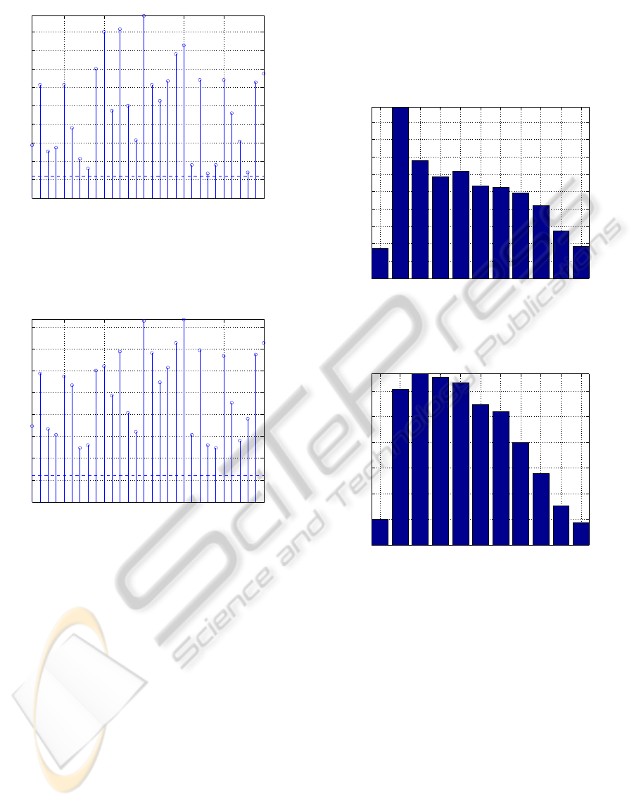
tails of the method. Fig. 1 and Fig. 2 show the test
set error rate of each feature obtained for the WBCD
dataset using the na¨ıve Bayes classifier, on discrete
features with the static U-LBG2 procedure with q = 4
and q = 8, respectively. We observe that the test set
error rates achieved individually by several features
are quite close to the error attained with the full set of
features (for example, features 8, 23, or 28 in Fig. 1).
Another interesting remark about Figs. 1 and 2 is that
increasing the number of bits per feature does not nec-
essarily lead to a decrease in the classification error;
again, if we look into the individual test set error rates
of features 8, 23, and 28, now with q = 8 bits (Fig. 2),
we observe an increase in the test set error rates with
respect to q = 4 bits (Fig. 1).
In order to gain insight into how the test set er-
ror rate of each feature evolves during discretization,
we compare the test set error rate of each feature with
its U-LBG2 discretized version with q ∈ {1, . . . , 10}.
Fig. 3 and Fig. 4 show the test set error rate of fea-
tures 17 and 25, again with the na¨ıve Bayes classifier,
respectively, for the WBCD dataset.
0 1 2 3 4 5 6 7 8 9 10
0
5
10
15
20
25
30
35
40
45
Error of feature 17 on WBCD
q (1 to 10) bits / feature ; 0 = Original feature
Err
Figure 3: Test set error rate of na¨ıve Bayes using solely
feature 17 of the WBCD dataset (original feature and U-
LBG2 discretized with q ∈ {1, . . . ,10}).
0 1 2 3 4 5 6 7 8 9 10
0
5
10
15
20
25
30
Error of feature 25 on WBCD
q (1 to 10) bits / feature ; 0 = Original feature
Err
Figure 4: Test set error rate of na¨ıve Bayes using solely
feature 25 of the WBCD dataset (original feature and U-
LBG2 discretized with q ∈ {1, . . . ,10}).
In the case of feature 17, discretization neverleads
to a lower test set error rate, as compared to the orig-
inal representation. On the other hand, for feature
25, the use of a larger number of bits leads to an im-
provement in the accuracy. These experimental re-
sults show typical situations that we observe with dif-
ferent types of data and depend on the statistics of
each feature, leading us to the following observations:
• some features are worth to be discretized up to
number of bits q;
• for other features, it is preferable not to discretize
them.
Algorithm 3 details our dynamic wrapper dis-
cretization (DWD) method. We use the following
notation: @class(X, y) denotes a function that learns
ICPRAM 2012 - International Conference on Pattern Recognition Applications and Methods
106

some classifier (e.g., support vector machine, na
¨
ıve
Bayes, K-nearest-neighbors) from the training set in
matrix X with labels y and returns the obtained er-
ror rate; @quant(·, b) denotes any of the unsupervised
(or supervised) scalar static discretization algorithms,
such as those mentioned above or any other, with b
bits. This algorithm performs its actions solely on the
training set portion of the data; it does not require the
existence of a separate hold-out test set.
Algorithm 3: DWD - Dynamic Wrapper Discretiza-
tion.
Input: X, n× p matrix training set (p features, n patterns).
y: n-length vector with class labels.
q: the maximum number of bits per feature.
@quant: a static discretizer.
@class: a supervised classifier.
Output:
e
X: n× p matrix, discretized version on X.
Q
1
, ..., Q
p
: set of p quantizers (one per feature).
1: for i = 1 to p do
2: err
i0
← @class(X
i
, y): training error rate using only
the i−th feature;
3: for b
i
= 1 to q do
4:
e
X
i
= @quant(X
i
, b
i
);
5: err
ib
← @class(
e
X
i
, y);
6: end for
7: end for
8: Find b
i
= arg min
j∈{0,1,...,q}
err
ij
, for i = 1,..., p.
9: for i = 1 to p do
10: if b
i
= 0 then
11:
e
X
i
= X
i
; {/* Don’t discretize the i-th feature */}
12: else
13: Q
i
(·) = @quant(·, b
i
); {/* Store quantizer*/}
14:
e
X
i
= Q
i
b
i
(X
i
);
15: end if
16: end for
In line 2, @class provides the baseline error, that
is, the training error rate with the original represen-
tation of each feature. A similar idea is applied in
line 5, where the classifier is applied to each dis-
cretized feature. Notice that if a discretized feature
never reaches a training error below the baseline, the
original representation is kept. We thus have a dy-
namic wrapper discretization procedure that produces
a hybrid dataset in the sense that it may contain both
discretized and non-discretized features. As a final
note on DWD (Algorithm 3), notice that the for loop
in line 3 does not need to start at b
i
= 1; we can set
the minimum number of bits per feature to some small
value, such as 3 or 4, thus computing fewer quantizers
and performing fewer evaluations.
3.3 Optimized Dynamic Discretization
For medium to high-dimensional datasets, the pro-
posed DWD method, as detailed in Algorithm 3, be-
comes computationally demanding. The need dis-
cretize each feature several times, and evaluate the
correspondingclassification accuracies, can make this
method prohibitive for higher dimensions (as it hap-
pens with many wrapper methods). The efficiency of
both the quantizer and the classifier is a key point to
avoid this computational burden. In order to decrease
the running time of our DWD algorithm, we havecon-
sidered that:
• the evolution of the test set error rates shown in
Fig. 1 and Fig. 2 suggest that for some features
there is no improvement on the classification per-
formance if we use a larger number of bits; more-
over, some (irrelevant) features will always lead
to low accuracy, regardless of the number of bits
we use for discretization;
• the results in Fig. 3 and Fig. 4, show that for some
features, there is no gain in discretizing them.
Combining these two ideas we propose the fol-
lowing optimization in order to delete the irrelevant
features as a pre-processing stage: after computing
the error of each feature, err
i0
← @class(X
i
, y) in line
2 of Algorithm 3, we keep only a fraction η of the
top rank features. We thus avoid the discretization of
many irrelevant features, saving execution time while
simultaneously improving the classification accuracy
and reducing the amount of memory needed to repre-
sent the dataset. This optimization can been seen as
wrapped FS process acting as a pre-processing stage
for the DWD algorithm; for this reason, we name
this optimized version of DWD as DWD-FS, being
a wrapper for both discretization and selection.
4 EXPERIMENTAL EVALUATION
This section reports experimental results obtained by
our FD techniques on several public domain datasets.
We use linear support vector machines (SVM), na
¨
ıve
Bayes (NB), and K-nearest-neighbors (KNN) (with
K = 3) classifiers, implemented in the PRTools
1
tool-
box (Duin et al., 2007). We start by assessing the
behavior of static discretization methods in Subsec-
tion 4.1 and proceed to the analysis of the dynamic
discretization methods in Subsection 4.2. In Subsec-
tion 4.3, we perform a running time analysis of these
methods. Finally, in Subsection 4.4, we apply FS
methods on the original and on the discretized fea-
tures to check if the discrete features lead to an in-
crease in the classification performance. The experi-
1
http://www.prtools.org/prtools.html
A DYNAMIC WRAPPER METHOD FOR FEATURE DISCRETIZATION AND SELECTION
107

Table 1: 11 UCI datasets and 5 microarray datasets used
in the experiments; p, c, and n are the number of features,
classes, and patterns, respectively.
Dataset Name p c n
Phoneme 5 2 5404
Pima 8 2 768
Abalone 8 2 4177
Contraceptve 9 2 1473
Wine 13 3 178
Hepatitis 19 2 155
WBCD 30 2 569
Ionosphere 34 2 351
SpamBase 54 2 4601
Lung 55 3 32
Arrhythmia 279 16 452
Colon 2000 2 62
SRBCT 2309 4 83
Lymphoma 4026 9 96
Leukemia 1 5327 3 72
9-Tumors 5726 9 60
ments were carried out on a common laptop computer
with 2.16 GHz CPU and 4 Gb of RAM.
Table 1 briefly describes the public domain bench-
mark datasets from the UCI Repository (Frank and
Asuncion, 2010) that were used in our experiments.
We chose several well-known datasets with different
kinds of data. We have also included public domain
microarray gene expression datasets
2
.
4.1 Analysis of Static Discretization
Fig. 5 shows the typical MSE decay obtained by the
U-LBG1 algorithm using up to q = 10 bits, when dis-
cretizing features 1 and 18 of the Hepatitis dataset.
This plot shows that even for features that start with a
high distortion (with a single bit), the MSE drops fast
(roughly exponentially fast).
Table 2 shows a comparison of three static FD
methods, namely EFB, U-LBG1, and U-LBG2 for
some standard datasets, using up to q = 7 bits. The
EIB method is not considered here, since it usually
attains poorer performance than the EFB method. For
each FD method, we show the average test set error
rate of the na¨ıve Bayes classifier for ten runs with dif-
ferent training/test replications and the total number
of bits allocated for the set of quantizers. Table 3
shows a similar set of results, using linear SVM clas-
sifiers. Comparing the results in Table 2 and Table 3,
we see that on these datasets, the linear SVM classi-
fiers attain better results than the na¨ıve Bayes classi-
fiers. In some cases, the linear SVM classifiers attains
better performance on the original features than on the
discretized ones. The EFB method has good results,
2
http://www.gems-system.org/
1 2 3 4 5 6 7 8 9 10
0
50
100
150
200
250
q (1 to 10) bits
MSE
MSE distortion on Hepatitis by U−LBG1
Feature 1
Feature 18
Figure 5: MSE evolution as a function of the number of bits
q ∈ {1, . . . , 10}, for the features 1 and 18 of the Hepatitis
dataset, using the U-LBG1 algorithm.
despite its simplicity; however, on microarray data
which we have a large number of features and a small
number of patterns (large p, small n) as well as multi-
class problems, the U-LBG methods tend to perform
better. Moreover, on the micoarray datasets, the na¨ıve
Bayes classifier performs poorly, so we don’t even re-
port those results.
4.2 Dynamic Discretization
We now compare static discretization versus DWD
and its optimized version DWD-FS, as described in
Subsection 3.3. Table 4 shows a comparison of the
static FD methods, EFB and U-LBG1 with their dy-
namic versions incorporated into our DWD method
(Algorithm 2), with linear SVM classifiers for wrap-
ping and evaluation.
The results in Table 4 suggest that the DWD
method tends to produce better results for datasets
with higher number of features. For low-dimensional
datasets, (roughly with p < 20), the additional com-
plexity of the dynamic wrapper method does not lead
to better results as compared to the static versions.
The DWD method tends to produce discrete repre-
sentations with a smaller number of bits, as compared
to the static counterparts. For the higher-dimensional
datasets in Table 4, the use of the DWD algorithm
generally improves the performance of the wrapper
static discretizer for both EFB an U-LBG1. The
Phoneme and Abalone datasets exhibit a behavior
such that the use of the original features is preferable;
none of the static or dynamic versions attains better
results.
Table 5 shows the test results of static, DWD, and
DWD-FS U-LBG2 discretization with q = 7 bits. For
the DWD-FS algorithm we keep the percentage η of
the top rank features; the choice of η leads to select m
features. In these tests, we use the KNN classifier.
ICPRAM 2012 - International Conference on Pattern Recognition Applications and Methods
108

Table 2: Total number of bits per pattern (T. Bits) and Test Set Error Rate (Err, average of ten runs, with different random
training/test partitions) for the static discretization methods, with up to q = 7 bits, using the na¨ıve Bayes classifier. The best
test set error rate is in bold face (in case of a tie, the best is considered the one with fewer bits).
EFB U-LBG1 U-LBG2
Dataset Original Err T. Bits Err T. Bits Err T. Bits Err
Phoneme 21.30 30 22.30 9 22.80 30 20.60
Pima 25.30 48 25.20 30 25.20 48 25.80
Abalone 28.00 48 27.60 15 27.20 48 27.70
Contraceptive 34.80 54 31.40 15 38.00 54 34.80
Wine 3.73 78 4.80 27 3.20 78 3.20
Hepatitis 20.50 95 21.50 32 21.00 39 18.00
WBCD 5.87 180 5.13 60 5.87 180 5.67
Ionosphere 10.60 198 9.80 49 17.40 198 11.00
SpamBase 15.27 324 13.40 54 15.73 324 15.67
Lung 35.00 318 35.00 74 35.83 318 35.00
Arrhythmia 32.00 1392 51.56 553 30.22 1392 41.56
Table 3: Total number of bits per pattern (T. Bits) and Test Set Error Rate (Err, average of ten runs, with different random
training/test partitions) for the static discretization methods, with up to q = 7 bits, using the linear SVM classifier. The best
test set error rate is in bold face (in case of a tie, the best is considered the one with less bits).
EFB U-LBG1 U-LBG2
Dataset Original Err T. Bits Err T. Bits Err T. Bits Err
Phoneme 22.60 30 24.00 8 21.80 30 22.70
Pima 27.50 48 28.50 27 29.30 48 27.60
Abalone 24.30 48 23.20 16 27.80 48 23.70
Contraceptive 36.50 54 34.60 15 39.80 54 37.20
Wine 4.80 78 1.87 25 5.33 78 1.33
Hepatitis 14.50 114 16.00 33 16.00 114 13.00
WBCD 4.67 180 3.07 59 2.80 180 2.80
Ionosphere 16.60 198 19.60 43 13.80 198 16.00
SpamBase 12.93 324 16.73 54 20.40 324 18.53
Lung 18.33 330 17.50 85 19.17 330 20.83
Arrhythmia 33.33 1392 31.78 550 32.89 1392 33.33
Colon 14.44 12000 11.11 9723 12.78 12000 10.56
SRBCT 0.00 13848 0.53 2793 0.20 13848 0.37
Lymphoma 0.57 24156 0.57 5910 0.00 24156 0.57
Leukemia1 11.43 26635 10.48 24306 5.71 26635 7.62
9-Tumors 22.22 28630 14.67 24906 12.00 28630 14.22
Table 4: Total number of bits per pattern (T. Bits) and Test Set Error Rate (Err, average of ten runs, with different random
training/test partitions) for the static and dynamic discretization methods for EFB and U-LBG1, with up to q = 7 bits, using
linear SVMs. The best test set error rate is in bold face (in case of a tie, the best is considered the one with fewer bits).
Static DWD Algorithm
EFB U-LBG1 EFB U-LBG1
Dataset Original Err T. Bits Err T. Bits Err T. Bits Err T. Bits Err
Phoneme 21.17 35 23.33 8 23.33 29 24.33 7 21.50
Pima 27.67 56 27.33 28 28.67 28 26.83 25 28.50
Abalone 23.00 56 24.67 16 27.67 26 25.33 13 26.00
Contraceptive 34.00 63 31.67 15 36.67 22 34.50 14 34.00
Wine 2.40 65 0.53 25 4.27 55 1.60 20 1.87
Hepatitis 20.50 95 21.50 32 21.00 39 18.00 29 19.00
WBCD 4.22 210 3.22 59 2.11 125 2.78 52 4.56
Ionosphere 13.40 165 20.00 43 13.00 126 18.40 40 12.40
SpamBase 14.20 260 15.87 52 17.73 82 11.87 52 14.20
Lung 22.22 371 23.61 76 25.00 81 22.22 65 22.22
These results show the adequacy of the DWD-FS
algorithm as compared to the other two. In the major-
ity of these tests, it attains the lowest test set error rate
using fewer features and fewer bits per feature; it thus
A DYNAMIC WRAPPER METHOD FOR FEATURE DISCRETIZATION AND SELECTION
109

Table 5: Total number of bits per pattern (T. Bits) and Test Set Error Rate (Err, average of ten runs, with different random
training/test partitions) for the static, DWD, and DWD-FS discretization methods for U-LBG2, with up to q = 7 bits, using
the KNN (K = 3) classifier. η is the percentage of the top rank features and m is the average number of features for the ten
runs. The best test set error rate is in bold face (in case of a tie, the best is considered the one with less bits).
Static U-LBG2 DWD U-LBG2 DWD-FS U-LBG2
Dataset Original Err T. Bits Err T. Bits Err η m T. Bits Err
Phoneme 22.15 35 22.35 35 22.15 0.8 4.0 28 21.90
Pima 26.10 56 26.10 50 26.00 0.8 6.0 40 27.00
Abalone 26.20 56 24.60 49 26.50 0.8 6.0 42 24.20
Contraceptive 44.60 63 45.30 13 45.50 0.8 7.0 11 43.60
Wine 27.20 91 6.13 84 14.67 0.8 10.0 65 12.27
Hepatitis 29.50 133 29.00 42 30.00 0.8 15.0 38 29.50
WBCD 7.07 210 3.93 209 6.93 0.8 24.0 167 3.80
Ionosphere 18.40 231 18.80 215 16.00 0.8 26.0 174 20.80
SpamBase 16.07 378 17.20 186 23.00 0.8 42.4 169 26.47
Lung 23.33 378 28.33 63 24.17 0.8 42.8 52 22.50
Table 6: Total time (in seconds) taken to discretize features
by the three static FD methods, namely EFB, U-LBG1, and
U-LBG2, using up to q = 7 bits. The fastest discretization
method is in bold face.
Dataset EFB U-LBG1 U-LBG2
Phoneme 0.20 0.27 0.79
Wine 0.09 0.05 0.14
Hepatitis 0.10 0.05 0.10
WBCD 0.24 0.29 0.86
SpamBase 0.32 0.07 0.40
Arrhythmia 1.23 0.96 1.55
Colon 11.66 21.81 18.12
SRBCT 32.60 23.57 52.57
Lymphoma 32.17 18.72 49.25
Leukemia 1 31.56 47.39 38.74
9-Tumors 43.49 64.85 55.77
leads to an improvement on the results of the KNN
classifier on both the original and U-LBG2 features.
The only test in which there are no benefits from the
discretization is on the sparse data SpamBase dataset;
in this case, the original features are preferable for the
KNN classifier.
4.3 Running Time Analysis
Table 6 shows a comparison of the time taken to dis-
cretize features by the three static FD methods, EFB,
U-LBG1, and U-LBG2, using up to q = 7 bits. The
U-LBG1 (Algorithm 1) also uses ∆ = 0.05range(X
i
).
These results show that the EFB and U-LBG2 tend
to take roughly the same time, allocating a maximum
of q bits per feature. The U-LBG1 algorithm usually
is faster since it stops before reaching the maximum
q bits; in fact, many features are discretized with a
number of bits much smaller than q.
Table 7 shows a similar comparison of the time
taken to discretize features by the DWD and DWD-
FS methods (with η = 0.8) using EFB discretization
and na¨ıve Bayes classifier, using up to q = 7 bits. The
Table 7: Time (in seconds) taken to discretize features by
EFB, DWD and DWD-FS methods (wrapped with EFB dis-
cretization and na¨ıve Bayes classifier), using up to q = 7
bits. We show the average time for ten runs.
Dataset EFB DWD EFB DWD-FS EFB
Phoneme 0.04 1.94 3.04
Wine 0.10 5.30 6.97
Hepatitis 0.09 7.01 9.80
WBCD 0.20 11.40 21.94
SpamBase 0.34 19.92 28.13
Arrhythmia 1.26 141.27 175.56
Colon 12.11 725.51 962.57
SRBCT 33.95 1270.97 1621.65
dynamic versions take much more time than the static
version. The choice of the classifier also influences
the time taken for the discretization. For medium to
high-dimensionaldatasets (p > 200), the implementa-
tions (without optimizations) of DWD and DWD-FS
are too time-consuming for practical applications.
4.4 Leveraging Feature Selection
In order to asses the quality (informativeness) of the
discretized features, we run a few tests using FS on
the original and on the discretized features. The key
idea of these tests is to show how the use of FS on the
discretized features can have benefits, as compared to
the original ones.
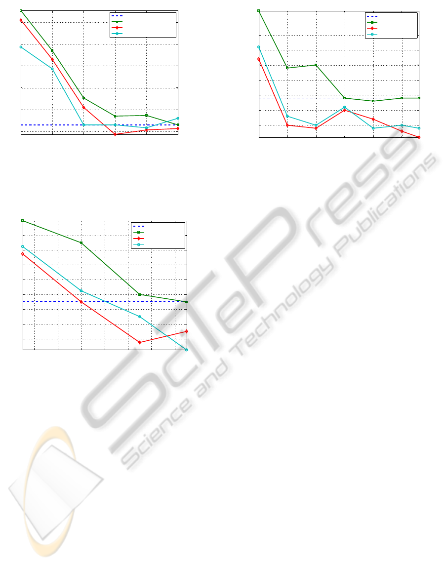
In Fig. 6, we report na¨ıve Bayes classifier test set
error rates with the features selected by the mrMR
method; we compare the original features with the
discretized versions obtained with the static and dy-
namic U-LBG1 methods. We observe that the use
discretized features seems to help the FS criterion,
since lower test error rates are achieved when com-
pared with the original ones.
In Fig. 7 and Fig. 8, we report na¨ıve Bayes test
set error rates with the features selected by the FiR
method, for the Hepatitis and the Ionosphere datasets,
ICPRAM 2012 - International Conference on Pattern Recognition Applications and Methods
110
5 10 15 20 25 30
6
7
8
9
10
11
m (# features)
Test set error rate on WBCD
Baseline
Original + mrMR
U−LBG1 Static + mrMR
U−LBG1 DWD + mrMR
Figure 6: Test set error rate (average of ten runs, with dif-
ferent training/test partitions), as functions of the number
of features, for the na¨ıve Bayes classifier, using FS by the
mrMR method, for the WBCD dataset on original, static,
and dynamically discretized features.
6 8 10 12 14 16 18
16
17
18
19
20
21
22
23
24
m (# features)
Error [%]
Test set error rate on Hepatitis
Baseline
Original + FiR
EFB Static + FiR
EFB DWD + FiR
Figure 7: Test set error rate (average of ten runs, with dif-
ferent training/test partitions), as functions of the number
of features, for the na¨ıve Bayes classifier, using FS by the
FiR method, for the Hepatitis dataset on original, static, and
dynamically discretized features.
respectively; we compare the original features with
the discretized versions obtained with the static and
dynamic EFB methods. For both datasets, the dis-
crete features are more adequate for FS as compared
to the original features.
5 CONCLUSIONS
In this paper, we have proposed static and dynamic
methods for feature discretization (FD). The static
method is unsupervised and the dynamic method uses
a wrapper approach with a quantizer and a classifier,
and it can be coupled with any static unsupervised (or
supervised) discretization procedure. The key idea of
the dynamic method is to assess the performance of
5 10 15 20 25 30
12
12.5
13
13.5
14
14.5
15
15.5
m (# features)
Error [%]
Test set error rate on Ionosphere
Baseline
Original + FiR
EFB Static + FiR
EFB DWD + FiR
Figure 8: Test set error rate (average of ten runs, with dif-
ferent training/test partitions), as functions of the number of
features, for the na¨ıve Bayes classifier, using FS by the FiR
method, for the Ionosphere dataset on original, static, and
dynamically discretized features.
each feature as discretization is carried out; if the orig-
inal representation is preferable to the discrete fea-
ture, then it is kept. An optimized version of this dy-
namic method uses a pre-processing stage which con-
sists in a wrapper feature selection process.
The proposed methods, equally applicable to bi-
nary and multi-class problems, attain efficient repre-
sentations, suitable for learning problems. Our exper-
imental results, on public-domain datasets with dif-
ferent types of data, show the competitiveness of our
techniques when compared with previous approaches.
The use of the features discretized by our methods
lead to better accuracy than using the original or dis-
cretized features by other methods.
As future work, we plan to optimize the imple-
mentation of our dynamic discretization method, and
to devise its filter version, suitable to tackle dynamic
discretization on (very) high-dimensional datasets.
REFERENCES
Clarke, E. and Barton, B. (2000). Entropy and MDL dis-
cretization of continuous variables for Bayesian be-
lief networks. International Journal of Intelligent Sys-
tems, 15(1):61–92.
Cover, T. and Thomas, J. (1991). Elements of Information
Theory. John Wiley & Sons.
Dougherty, J., Kohavi, R., and Sahami, M. (1995). Super-
vised and unsupervised discretization of continuous
features. In International Conference Machine Learn-
ing — ICML’95, pages 194–202. Morgan Kaufmann.
Duin, R., Juszczak, P., Paclik, P., Pekalska, E., Ridder, D.,
Tax, D., and Verzakov, S. (2007). PRTools4.1: A Mat-
lab Toolbox for Pattern Recognition. Technical report,
Delft Univ. Technology.
A DYNAMIC WRAPPER METHOD FOR FEATURE DISCRETIZATION AND SELECTION
111

Escolano, F., Suau, P., and Bonev, B. (2009). Information
Theory in Computer Vision and Pattern Recognition.
Springer.
Fayyad, U. and Irani, K. (1993). Multi-interval discretiza-
tion of continuous-valued attributes for classification
learning. In Proceedings of the International Joint
Conference on Uncertainty in AI, pages 1022–1027.
Ferreira, A. and Figueiredo, M. (2011). Unsupervised joint
feature discretization and selection. In 5th Iberian
Conference on Pattern Recognition and Image Analy-
sis - IbPRIA2011, pages 200–207, Las Palmas, Spain.
Frank, A. and Asuncion, A. (2010). UCI machine learning
repository, available at http://archive.ics.uci.edu/ml.
Furey, T., Cristianini, N., Duffy, N., Bednarski, D., Schum-
mer, M., and Haussler, D. (2000). Support vector
machine classification and validation of cancer tissue
samples using microarray expression data. Bioinfor-
matics, 16(10):906–914.
Guyon, I. and Elisseeff, A. (2003). An introduction to vari-
able and feature selection. Journal of Machine Learn-
ing Research, 3:1157–1182.
Guyon, I., Gunn, S., Nikravesh, M., and Zadeh (Editors), L.
(2006). Feature Extraction, Foundations and Applica-
tions. Springer.
Hastie, T., Tibshirani, R., and Friedman, J. (2009). The El-
ements of Statistical Learning. Springer, 2nd edition.
Kotsiantis, S. and Kanellopoulos, D. (2006). Discretization
techniques: A recent survey. GESTS International
Transactions on Computer Science and Engineering,
32(1).
Linde, Y., Buzo, A., and Gray, R. (1980). An algorithm for
vector quantizer design. IEEE Trans. on Communica-
tions, 28:84–94.
Liu, H., Hussain, F., Tan, C., and Dash, M. (2002). Dis-
cretization: An Enabling Technique. Data Mining and
Knowledge Discovery, 6(4):393–423.
Meyer, P., Schretter, C., and Bontempi, G. (2008).
Information-theoretic feature selection in microarray
data using variable complementarity. IEEE Journal
of Selected Topics in Signal Processing (Special Is-
sue on Genomic and Proteomic Signal Processing),
2(3):261–274.
Peng, H., Long, F., and Ding, C. (2005). Feature selec-
tion based on mutual information: Criteria of max-
dependency, max-relevance, and min-redundancy.
IEEE Transactions on Pattern Analysis and Machine
Intelligence, 27(8):1226–1238.
Tsai, C.-J., Lee, C.-I., and Yang, W.-P. (2008). A dis-
cretization algorithm based on class-attribute contin-
gency coefficient. Inf. Sci., 178:714–731.
Witten, I. and Frank, E. (2005). Data Mining: Practical
Machine Learning Tools and Techniques. Elsevier,
Morgan Kauffmann, 2nd edition.
Yu, L., Liu, H., and Guyon, I. (2004). Efficient feature
selection via analysis of relevance and redundancy.
Journal of Machine Learning Research, 5:1205–1224.
Zhu, Q., Lin, L., Shyu, M., and Chen, S. (2011). Effective
supervised discretization for classification based on
correlation maximization. In IEEE International Con-
ference on Information Reuse and Integration (IRI),
pages 390–395, Las Vegas, Nevada, USA.
ICPRAM 2012 - International Conference on Pattern Recognition Applications and Methods
112
