
LEAST-SQUARES ESTIMATION OF NANOPORE CHANNEL
CONDUCTANCE IN VOLTAGE-VARYING EXPERIMENTS
Christopher R. O’Donnell and William B. Dunbar
Baskin School of Engineering, University of California, Santa Cruz, U.S.A.
Keywords:
Nanopore, Single Channel Recording, Least-squares, Online Parameter Estimation, State-space Modeling.
Abstract:
Step-changing and sinusoidal voltage patterns have expanded the capabilities of the nanopore instrument for
single molecule manipulation and measurement. A challenge with voltage-varying experiments is that capaci-
tance in the system is excited and masks the contribution of the nanopore channel conductance in the measured
current. The conductance is the parameter that can be used to infer the dynamics of the complex (e.g., DNA, or
DNA-protein) in the pore. We present a least-squares parameter estimation (LSPE) algorithm for estimating
the channel conductance under voltage-varying conditions, including step and sinusoidal voltages, with the
objective of inferring the channel conductance parameter as continuously as possible. The algorithm is shown
to recover the conductance faster than by waiting for capacitive transients to settle in step-voltage experiments,
and provides accurate continuous conductance estimates in sinusoidal voltage experiments, with realistic noise
levels superimposed on the measurements.
1 INTRODUCTION
Nanoscale pores are an established tool for measuring
and manipulating individual DNA and DNA-protein
complexes (Wilson et al., 2009), (Olasagasti et al.,
2010). The nanopore device modeled in this work,
shown in Figure 1, consists of a single α-hemolysin
protein channel inserted in a lipid bilayer, which sep-
arates two chambers containing a bufferedelectrolytic
solution. Voltage is applied across the bilayer creat-
ing an ionic current through the nanopore that is mea-
sured and passed through a 4-pole Bessel filter before
being sampled and recorded. As DNA molecules are
captured and driven through the nanopore, the con-
ductance of the channel is reduced causing a drop in
the measured ionic current. This change in current (or
conductance) and its duration are used to characterize
the state of the molecule captured in the nanopore.
Constant voltages have been used in the past to
examine DNA and enzyme-bound DNA complexes
(Benner et al., 2007). The use of time-varying volt-
ages has expanded the capabilities of the nanopore.
For example, active control with step-changing volt-
ages has been used to measure nanopore-DNA in-
teractions (Bates et al., 2003), and polymerase-DNA
interactions on the nanopore (Wilson et al., 2009),
(Olasagasti et al., 2010), at the single molecule level.
Sinusoidal voltage patterns have also made it possi-
ble to monitor the presence of DNA in the pore at
zero DC voltage (Ervin et al., 2008), with the assis-
tance of custom hardware and filtering. A challenge
with time-varying voltages is that the capacitive ele-
ments in the system contribute to the measured ionic
current. In step-changing experiments, the true value
of the conductance is obscured for the duration of the
transient, restiricting the time-resolution limits for de-
tecting DNA or DNA-protein dynamics (Wilson et al.,
2009). The LSPE algorithm presented in this paper
uses the classical method of least-squares approxi-
mation. The derived LSPE is shown to provide ef-
ficient online estimation of the channel conductance
during step-changing voltages, and continuous esti-
mation during sinusoidal voltage inputs, with realistic
noise superimposed on the measurements.
2 NANOPORE SYSTEM MODEL
The four-state model of the nanopore system has the
transfer function H(s) from the input voltage V
p
to
the output current I
p
(i.e., I
p
(s)/V
p
(s) = H(s) in the
Laplace domain) given by
H(s) =
C
Σ
s+ G
c
a
1
s
4
+ a
2
s
3
+ a
3
s
2
+ a
4
s+ 1
270
O’Donnell C. and Dunbar W..
LEAST-SQUARES ESTIMATION OF NANOPORE CHANNEL CONDUCTANCE IN VOLTAGE-VARYING EXPERIMENTS.
DOI: 10.5220/0003790502700275
In Proceedings of the International Conference on Bio-inspired Systems and Signal Processing (BIOSIGNALS-2012), pages 270-275
ISBN: 978-989-8425-89-8
Copyright
c
2012 SCITEPRESS (Science and Technology Publications, Lda.)

R
c
C
m
R
a
V
p
V
Control
Logic
A
Amplifier
Voltage
pattern
(step, sine)
Current
response
LSPE
G
c
^
≈1/R
c
C
p
Figure 1: An amplifier applies voltage and measures the
ionic current through the nanopore channel. Control logic
is used to monitor the current and control the input volt-
age pattern. The known input signal and the measured cur-
rent response are used by the LSPE algorithm to estimate
b
G
c
≈ G
c
= 1/R
c
, the conductance of the nanopore channel.
In the circuit model of the system, R
c
is the resistance of the
channel, C
m
and C
p
are the membrane and parasitic capac-
itances, respectively, V
p
is the voltage at the output of the
amplifier, and R
a
is the electrolytic access resistance.
whereC
Σ
= C
p
+C
m
(pF) is the combined capacitance
of the system (Fig. 1), G
c
(nS) is the channel con-
ductance of the nanopore and the coefficients a
1
, a
2
,
a
3
and a
4
are characteristic of the Bessel filter. For
consistency of units, time is in milliseconds and fre-
quency is in kHz. We can ignore R
a
in the model
since it is negligible (∼ 10
−4
GΩ) compared to R
c
(3
GΩ). In another work, we have used system identifi-
cation tools to validate this model with experimental
data (Garalde et al., 2011). The coefficients are de-
fined in terms of the −3 dB cutoff frequency f
c
as
(a
1
,a
2
,a
3
,a
4
) =
(1,10f,45f
2
,105f
3
)
105f
4
, (1)
with f = (2π f
c
)/2.113917675 (numerator constant
identified to match f
c
with −3 dB frequency). The
frequencydomain representation of the system is con-
verted to continuous time state-space (control canon-
ical) form:
˙x(t) = Ax(t) + Bu(t), y(t) = Cx(t); t ≥ 0 (2)
with column vector x = [x
1
;x
2
;x
3
;x
4
] and matrices
A =
0 1 0 0
0 0 1 0
0 0 0 1
−1/a
1
−a
4
/a
1
−a
3
/a
1
−a
2
/a
1
,
B =
0
0
0
1
and C =
G
c
/a
1
C
Σ
/a
1
0 0
.
In the simulations in Section 4, white noise is added
to u and y (with different variances). The system
model (2) and LSPE algorithm can be extended to in-
corporate explicit models of noise (white or colored),
with such noise models being experimentally identi-
fied. This extension is not done here for brevity.
2.1 Time Discretization of Equations
To perform estimation of parameter G
c
by least-
squares, the continuous equations of the model are
first discretized. The solution to (2) is
x(t) = e
At
x(0) +
Z
t
0
e
A(t−τ)
Bu(τ)dτ
y(t) = Ce
At
x(0) +
Z
t
0
Ce
A(t−τ)
Bu(τ)dτ.
The sample period ∆ defines sample times t
k
= k ∗ ∆.
The input signal is assumed to be piece-wise con-
stant between the sample times: u(t) = u(t
k
) for all
t ∈ [t
k
,t
k+1
). Using this, the continuous solution is
converted to discrete time form as
x(t
k+1
) = A
d
x(t
k
) + B
d
u(t
k
), y(t
k
) = C
d
x(t
k
), (3)
with A
d
= e
A∆
, B
d
=
R
∆
0
e
A(∆−τ)
dτ
B, and C
d
= C.
The matrix A is invertible, so the matrix B
d
can be
rewritten as B
d
= A
−1
e
A∆
− I
B.
2.1.1 Delta Operator Form
Equation (3) is the traditional discrete time shift oper-
ator form, which models the absolute displacement of
the state vector from sample to sample, whereas equa-
tion (2) models the infinitesimal increment of the state
vector defined by the time derivative. This underly-
ing characteristic of the continuous time state-space
equations is more accurately modeled in discrete time
using the delta operator form (Goodwin et al., 1992).
Also known as the divided difference operator form,
the delta operator form models the change in the ab-
solute displacement of the state vector from sample
to sample over a given sample period. Using the delta
operator, the discrete time state-space model takes the
form
x
δ
(t
k
) = A
δ
x(t
k
) + B
δ
u(t
k
)
x(t
k+1
) = x(t
k
) + x
δ
(t
k
)∆
y(t
k
) = C
δ
x(t
k
),
(4)
with A
δ
= (A
d
− I)/∆, B
δ
= B
d
/∆, and C
δ
= C
d
= C.
Equation (4) is used in the remainder of the paper
to construct the LSPE algorithm and simulate the re-
sponse of the nanopore system.
3 LEAST-SQUARES PARAMETER
ESTIMATION (LSPE)
ALGORITHM
Algebraically, the sampled output can be written in
terms of the system parameters, the state vector and
LEAST-SQUARES ESTIMATION OF NANOPORE CHANNEL CONDUCTANCE IN VOLTAGE-VARYING
EXPERIMENTS
271

the initial condition by recursively evaluating equa-
tion (4). Beginning with t
1
, the solution of the sam-
pled output at t
n
takes the form
y(t
n
) =
G
c
a
1
"
x
1
(t
0
) +
n−1
∑
i=0
x
δ,1
(t
i
)∆
#
+
C
Σ
a
1
"
x
2
(t
0
) +
n−1
∑
i=0
x
δ,2
(t
i
)∆
#
(5)
The matrix expression of interest that relates the out-
put to the system parameters G
c
and C
Σ
can now be
defined as
y(t
1
)
y(t
2
)
.
.
.
y(t
n
)
=
Q
1
Q
2
G
c
/a
1
C
Σ
/a
1
with
Q
1
=
x
1
(t
0
) + x
δ,1
(t
0
)∆
x
1
(t
0
) + x
δ,1
(t
0
)∆+ x
δ,1
(t
1
)∆
.
.
.
x
1
(t
0
) +
∑
n−1
i=0
x
δ,1
(t
i
)∆
and
Q
2
=
x
2
(t
0
) + x
δ,2
(t
0
)∆
x
2
(t
0
) + x
δ,2
(t
0
)∆+ x
δ,2
(t
1
)∆
.
.
.
x
2
(t
0
) +
∑
n−1
i=0
x
δ,2
(t
i
)∆
which is written in vector notation as
y
1,n
= Qz
where the matrix Q = [Q
1
Q
2
] ∈ R
n×2
and the column
vector z = [G
c
/a
1
; C
Σ
/a
1
] ∈ R
2
.
3.1 Least-squares Solution
The least-squares approximation problem is based
upon finding the best estimate ˆz of the vector z that
minimizes
kQz− y
1,n
k
2
where k · k represents the Euclidean norm. Since the
matrix Q has more rows than columns and has full
column rank, the least-squares approximation prob-
lem has a unique solution (Boyd and Vandenberghe,
2004) in the form
ˆz = (Q
T
Q)
−1
Q
T
y
1,n
.
Once the least-squares solution ˆz is computed, the es-
timates of the channel conductance and the system ca-
pacitance are [
b
G
c
;
b
C
Σ
] = ˆz× a
1
.
3.2 Sequential Implementation
The channel conductance of the nanopore changes
when DNA is captured and translocates through the
nanopore. These capture events occur on a micro-to-
millisecond time scale (Benner et al., 2007). Thus, the
LSPE algorithm must be able to estimate changes in
G
c
on these time scales. This is accomplished through
sequential implementation of the algorithm on over-
lapping windows of length n that span the input and
output data sets of length N, where N ≫ n. We fo-
cus on an online implementation here that makes use
of past windows of data to generate the estimate
b
G
c
.
Offline implementation is acceptable when detecting
protein-DNA dissociation events after an active con-
trol experiment is run, while online implementation
allows superior active control during an experiment
(Wilson et al., 2009), (Olasagasti et al., 2010).
Sequential implementation of the LSPE algorithm
requires the initial condition x(t
0
) used in equation (5)
to be reset after each iteration to reflect the starting
point of the next window. This requires knowledge
of the state vector x at every sample instance, which
presents a problem since x cannot be directly mea-
sured or calculated from measurements. This problem
is overcome by simulating x at every sample instance
using the system model (4) with a known input signal.
4 RESULTS AND DISCUSSION
The performance of the LSPE algorithm was tested in
simulations with step-changing and sinusoidal volt-
ages. To emulate realistic experimental conditions,
white noise was added to the input (0.2 mV RMS) and
filtered output (1.5 pA RMS) with variances close to
those observed experimentally (Wilson et al., 2009)
(noise is white up to 10 kHz bandwidth). Also, the
value of G
c
was set to 1/3 nS for positive voltages
and 2/9 nS for negative voltages, consistent with val-
ues for experiments performed in 0.3 M KCl buffered
solution (Wilson et al., 2009). The performance of
the LSPE algorithm is compared here to the perfor-
mance of a simple “I/V method,” defined as estimat-
ing the conductance by I
p
(t
k
)/V
p
(t
k
) at each sample
time t
k
. When voltage is constant, the current is con-
stant unless changes in G
c
occur, for example, if DNA
is captured in the nanopore, or polymerase bound to
DNA dissociates from the DNA (Wilson et al., 2009),
(Olasagasti et al., 2010). Thus, when V
p
is constant
for a sustained period, the I/V method produces an
accurate estimate for G
c
. To be of value in estimating
G
c
, the LSPE should perform comparably to the I/V
method when V
p
is constant, and outperform the I/V
BIOSIGNALS 2012 - International Conference on Bio-inspired Systems and Signal Processing
272

method when V
p
is time-varying.
4.1 Step-changing Input
For a step-changing input, the output current stays
constant except when the input transitions from one
level to another. The switching of the input voltage
produces a transient response in the output current,
the duration of which is dependent on the amplitude
of the input voltage, the amount of capacitance in the
systemC
Σ
and the Bessel filter cutofffrequency f
c
. Of
these three effects, the post-step-change settling time
of the LSPE algorithm is most sensitive to the value of
f
c
. An increase from 1 kHz to 10 kHz bandwidth re-
duces the time it takes the algorithm to settle to within
90% of its steady-state value from 0.996 ms to 0.212
ms (data not shown). However, in the presence of ad-
ditive noise, larger bandwidth also allows more noise
to contaminate the estimate
b
G
c
. To mitigate this trade-
off between minimizing settling time and minimizing
the standard deviation of the estimate, f
c
= 1 kHz was
qualitatively chosen as the optimal bandwidth for the
LSPE algorithm. Settling time of the algorithm is
also effected by the length n of the sequential over-
lapping windows. Smaller n enables the algorithm
to more efficiently track the true value of G
c
, but al-
lows more noise to contaminate the estimate. Again,
to mitigate the tradeoff between minimizing settling
time and standard deviation, n = 250 was chosen in
this paper. Future work will determine quantitative
metrics for establishing the optimal f
c
and n choices.
Without noise and at 1 kHz bandwidth and 250
kHz sample rate, the step-response settling time of
the LSPE estimate
b
G
c
is 0.996 ms, compared to 1.412
ms for the I/V method. That is, the LSPE estimate
converges faster (70%) than the output current does.
Practically, capacitance compensation on the record-
ing amplifier can speed the current settling time (and
thus the I/V method’s estimate). However, the I/V
method with a compensated current will, in general,
not work in both step and sinusoidal conditions with-
out heuristic tuning of the compensation settings for
each set of conditions (voltage pattern, bandwidth),
while the LSPE algorithm works universally.
The performance of the LSPE algorithm for step
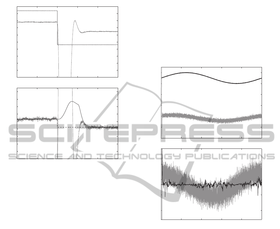
voltages is shown in Figures 2 and 3. In Figure 2, the
20 mV voltage step is always positive so G
c
= 1/3
nS. The LSPE estimate
b
G
c
has a much smaller stan-
dard deviation, and the I/V method produces a much
larger overshoot. In Figure 3, the 240 mV voltage step
changes polarity, causing a step change in G
c
from
1/3 to 2/9 nS. The LSPE algorithm has a larger over-
shoot than in the previous case, but the I/V method
estimate still has a larger overshoot and standard de-
viation at steady-state. In these voltage changes, we
ignore saturation of the measurement current, which
can occur if the recorded output gain is set to high.
Future work will examine and mitigate the effect of
output saturation for the LSPE algorithm.
The LSPE algorithm outperforms the I/V method
in that the estimate
b
G
c
has a smaller standard devia-
tion. One might argue that the LSPE algorithm is sim-
ply acting as a filter, and the performance of the I/V
method could be improved if the current were first fil-
tered. In fact, the LSPE algorithm is not a filter but an
estimator, recursively computing the value of
b
G
c
that
minimizes the error between the measured currentand
current modeled by (4). Although additional low-pass
filtering of the current would reduce the standard de-
viation of the I/V estimate, the filter would further in-
crease the settling time of the estimate.
48 49 50 51 52 53
0.25
0.3
0.35
0.4
0.45
Time (ms)
ˆ
G
c
(nS)
48 49 50 51 52 53
−350
−300
−250
−200
−150
−100
−50
0
50
100
150
Time (ms)
Input (mV), Output (pA)
A
B
Input Voltage
Output Current
I/V
LSPE
Figure 2: A) Voltage step response (120 to 100 mV) of the
nanopore system model. B) A comparison of the LPSE
and I/V methods for generating
b
G
c
. The I/V method has
a larger steady-state standard deviation (1.36 × 10
−2
nS)
and a much larger overshoot (3.669 nS) in response to a
step change than the LSPE algorithm (7.927× 10
−4
nS and
9.708× 10
−3
nS).
4.2 Sinusoidal Input
For a sinusoidal voltage input, the output current is
constantly in a transient state, with the capacitive
elements in the system being persistently excited.
This has a positive effect on the LSPE algorithm in
LEAST-SQUARES ESTIMATION OF NANOPORE CHANNEL CONDUCTANCE IN VOLTAGE-VARYING
EXPERIMENTS
273
48 49 50 51 52 53
−0.2
−0.1
0
0.1
0.2
0.3
0.4
0.5
0.6
0.7
Time (ms)
ˆ
G
c
(nS)
48 49 50 51 52 53
−350
−300
−250
−200
−150
−100
−50
0
50
100
150
Time (ms)
Input (mV), Output (pA)
A
B
Input Voltage
Output Current
I/V
LSPE
Figure 3: A) Voltage step response (120 to −120 mV) of the
nanopore system model. B) A comparison of the LPSE and
I/V methods for generating
b
G
c
. The voltage sign change at
50 ms causes a step change in G
c
from 1/3 to 2/9 nS. The
two methods have comparable settling times, with the LSPE
algorithm having a smaller steady-state standard deviation
(8.898 × 10
−4
nS) and overshoot (0.349 nS) than the I/V
method (1.34× 10
−2
nS and 36.57 nS).
that once
b
G
c
converges, it does not diverge again,
even though both input and output signals are non-
constant. The settling time of
b
G
c
is insensitive to
changes in the sinusoidal frequency f
w
. The standard
deviation of the estimate increases modestly from
2.69
−2
nS to 3.49 × 10
−2
nS as f
w
decreases from
10 Hz to 1 Hz. The sinusoidal frequency f
w
= 10 Hz
is used in the remainder of the paper.
The I/V method does not produce accurate values
of
b
G
c
for sinusoidal voltages, as expected, but we re-
port the comparison here. Future work will compare
LSPE to impedance spectroscopy methods (Katz and
Willner, 2003). These methods are comparable to our
estimator, and are designed specifically for sinusoidal
voltage inputs. The performance of the LSPE algo-
rithm for sinusoidal input voltages is shown in Fig-
ures 4 and 5. In Figure 4, G
c
= 1/3 nS since the input
stays positive. The I/V estimate has a large standard
deviation and follows a 10 Hz sinusoidal pattern of
the measurements, never converging to G
c
. The I/V
estimate crosses the true value of G
c
only at the peaks
of the sinusoidal input voltage. This also holds for a
sinusoidal input that changes polarity, shown in Fig-
ure 5. The change in polarity results in a step change
in G
c
, which the LSPE algorithm tracks well (Fig. 5).
The LSPE estimate is noisier than when voltage re-
mains positive (Fig. 4), but remains centered around
the true values of G
c
(1/3 nS and 2/9 nS), whereas
the I/V estimate ranges between 3.6 × 10
3
nS and
−2.1× 10
−4
nS.
0 20 40 60 80 100
0.25
0.3
0.35
0.4
0.45
Time (ms)
ˆ
G
c
(nS)
0 20 40 60 80 100
0
20
40
60
80
100
120
Time (ms)
Input (mV), Output (pA)
Input Voltage
Output Current
I/V
LSPE
A
B
Figure 4: A) Sinusoidal voltage response (10 mV peak-to-
peak, 10 Hz, 110 mV DC offset) of the nanopore system
model. B) A comparison of the LPSE and I/V methods
for generating
b
G
c
. The I/V method’s estimate has a larger
standard deviation (2.8×10
−2
nS) than the LSPE algorithm
(5.4× 10
−3
nS) and does not generate accurate estimates.
5 CONCLUSIONS
The LSPE algorithm presented in this paper provides
an accurate means for estimating the channel con-
ductance of a nanopore under voltage-varying con-
ditions. The algorithm consistently achieves better
performance (in terms of convergence time and stan-
dard deviation of the estimate) than the simple I/V
method for both step-changing and sinusoidal input
voltages. Since variance is improved, DNA or DNA-
protein events that can be detected by the measured
current (i.e., there is sufficient single-to-noise ratio)
are easier to detect with our LSPE algorithm.
We focused on an online implementation here that
BIOSIGNALS 2012 - International Conference on Bio-inspired Systems and Signal Processing
274

0 20 40 60 80 100
−0.2
−0.1
0
0.1
0.2
0.3
0.4
0.5
0.6
0.7
Time (ms)
ˆ
G
c
(nS)
0 20 40 60 80 100
−150
−100
−50
0
50
100
150
Time (ms)
Input (mV), Output (pA)
A
B
Input Voltage
Output Current
I/V
LSPE
Figure 5: A) Sinusoidal voltage response (120 mV peak-
to-peak, 10 Hz, 0 mV DC offset) of the nanopore system
model. B) A comparison of the LPSE and I/V methods for
generating
b
G
c
. The voltage sign change at 50 ms causes
a step change in G
c
from 1/3 to 2/9 nS. The I/V method
does not generate accurate estimates, whereas the LSPE al-
gorithm does track the change in G
c
.
uses fixed-length windows of past data to generate
the estimated conductance value. Future work will
explore improving the algorithm’s performance by
varying the window length based on detected rates of
change of the data (Jiang and Zhang, 2004), and by
incorporating forgetting-factors in the sequential im-
plementation (Ljung and Gunnarsson, 1990). Also,
an offline implementation that makes use of future
windows to compute the estimate will be developed
to further improve the detection resolution of rapid
DNA-protein dissociation events that follow voltage
changes in active control experiments (Wilson et al.,
2009), (Olasagasti et al., 2010).
The cited advantage of AC-signal detection (ab-
sent DC bias) is that nanopore/analyte interactions
can be measured while reducing the effects of elec-
troosmosis, electrophoresis, and protein deformation
that accompany large DC biases (Ervin et al., 2008).
In (Ervin et al., 2008), custom hardware (lock-in am-
plifier) and software permit high frequency (10–20
mV, 1–2 kHz f
w
) sinusoidal voltage inputs. The LSPE
derived here cannot track G
c
at sinusoidal frequencies
above 50 Hz (data not shown). Future work will ex-
plore if and how well the LSPE estimate may track
the presence of DNA in the pore at sinusoidal volt-
ages around 0 mV (no DC bias), at 5–50 Hz frequen-
cies, as an alternative to the high frequency method in
(Ervin et al., 2008).
REFERENCES
Bates, M., Burns, M., and Meller, A. (2003). Dynamics
of DNA molecules in a membrane channel probed
by active control techniques. Biophysical Journal,
84:2366–2372.
Benner, S., Chen, R. J. A., Wilson, N. A., Abu-Shumays,
R., Hurt, N., Lieberman, K. R., Deamer, D. W., Dun-
bar, W. B., and Akeson, M. (2007). Sequence-specific
detection of individual DNA polymerase complexes in
real time using a nanopore. Nature Nanotechnology,
2:718–724.
Boyd, S. P. and Vandenberghe, L. (2004). Convex Optimiza-
tion. Cambridge University Press.
Ervin, E. N., Kawano, R., White, R., and White, H. (2008).
Simultaneous alternating and direct current readout
of protein ion channel blocking events using glass
nanopore membranes. Anal. Chem, 80(6):2069–2076.
Garalde, D. R., Maitra, R. D., O’Donnell, C. R., Wang,
G., and Dunbar, W. B. (2011). Modeling the biolog-
ical nanopore instrument for biomolecular state esti-
mation. IEEE Trans. on Control Systems Technology,
in preparation.
Goodwin, G. C., Middleton, R. H., and Poor, H. V. (1992).
High-speed digital signal processing and control. Pro-
ceedings of the IEEE, 80(2):240–259.
Jiang, J. and Zhang, Y. (2004). A novel variable-length
sliding window blockwise least-squares algorithm for
on-line estimation of time-varying parameters. Inter-
national Journal of Adaptive Control and Signal Pro-
cessing, 18(6):505–521.
Katz, E. and Willner, I. (2003). Probing biomolecular inter-
actions at conductive and semiconductive surfaces by
impedance spectroscopy: Routes to impedimetric im-
munosensors, DNA-sensors, and enzyme biosensors.
Electroanalysis, 15(11):913–947.
Ljung, L. and Gunnarsson, S. (1990). Adaptation and track-
ing in system identification—a survey. Automatica,
26(1):7–21.
Olasagasti, F., Lieberman, K. R., Benner, S., Cherf, G. M.,
Dahl, J. M., Deamer, D. W., and Akeson, M. (2010).
Replication of individual DNA molecules under elec-
tronic control using a protein nanopore. Nature Nan-
otechnology, 5(11):798–806.
Wilson, N. A., Abu-Shumays, R., Gyarfas, B., Wang, H.,
Lieberman, K. R., Akeson, M., and Dunbar, W. B.
(2009). Electronic control of DNA polymerase bind-
ing and unbinding to single DNA molecules. ACS
Nano, 3:995–1003.
LEAST-SQUARES ESTIMATION OF NANOPORE CHANNEL CONDUCTANCE IN VOLTAGE-VARYING
EXPERIMENTS
275
