
SINGLE-FRAME SIGNAL RECOVERY USING A
SIMILARITY-PRIOR BASED ON PEARSON TYPE VII MRF
Sakinah Ali Pitchay and Ata Kab´an
School of Computer Science, University of Birmingham, Edgbaston, Birmingham, B15 2TT, U.K.
Keywords:
Single frame super-resolution, Compressive sensing, Similarity prior, Image recovery.
Abstract:
We consider the problem of signal reconstruction from noisy observations in a highly under-determined prob-
lem setting. Most of previous work does not consider any specific extra information to recover the signal.
Here we address this problem by exploiting the similarity between the signal of interest and a consecutive
motionless frame. We incorporate this additional information of similarity that is available into a probabilistic
image prior based on the Pearson type VII Markov Random Field model. Results on both synthetic and real
data of MRI images demonstrate the effectiveness of our method in both compressed setting and classical
super-resolution experiments.
1 INTRODUCTION
Conventional image super-resolution (SR) aims to re-
cover a high resolution scene from a single or multi-
ple frames of low resolution measurements. A noisy
frame of a single low resolution image or signal often
suffers from a blur and down-sampling transforma-
tion. The problem is more challenging when the ob-
served data is a single low resolution frame because
it contains fewer measurements than the number of
unknown pixels of the high resolution scene that we
aim to recover. This makes the problem ill-posed and
under-determined too. For this reason, some addi-
tional prior knowledge is vital to obtain a satisfactory
solution. We have demonstrated in previous work (A.
Kab´an and S. AliPitchay, 2011) that the Pearson type
VII density integrated with Markov Random Fields
(MRF) is an appropriate approach for this purpose.
In this paper, we tackle the problem using a more
specific prior information, namely the similarity to a
motionless consecutive frame as the additional input
for recovering the signals of interest in a highly under-
determined setting. This has real applications e.g.
in medical imaging where such frames are obtained
from several scans. Previous work in (N. Vaswani
and W. Lu, 2010) found the average frame from those
scans to be useful for recovery.
In principle, the more information we have about
the recovered signal, the better the recovery algorithm
is expected to perform. This hypothesis seems to
work in (JCR. Giraldo et al., 2010; N. Vaswani and
W. Lu, 2010), however both of these works require
us to tune the free parameters of the model manu-
ally, and (JCR. Giraldo et al., 2010) reckons that the
range of parameter values was not exhaustivelytested.
(N. Vaswani and W. Lu, 2010) also mentions that
they were not able to attain exact reconstruction us-
ing fewer measurements than those needed by com-
pressed sensing (CS) for a small image. By contrary,
in this paper we will demonstrate good recovery from
very few measurements using a probabilistic model
that includes an automated estimation of its hyper-
parameters.
Related work on sparse reconstruction gained
tremendous interest recently and can be found in e.g.
(R. G. Baraniuk et al., 2010; S. Ji et al., 2008; E. Can-
des et al., 2006; DL. Donoho, 2006). The sparser a
signal is, in some basis, the fewer random measure-
ments are sufficient for its recovery. However these
works do not consider any specific extra information
that could be used to accentuate the sparsity, which is
our focus. Somewhat related, the recent work in (W.
Lu and N. Vaswani, 2011) exploits partial erroneous
information to recover small image sequences.
This paper is aimed at taking these ideas further
through a more principled and more comprehensive
treatment. We consider the case when the observed
frame contains too few measurements, but an addi-
tional motionless consecutive scene in high resolu-
tions is provided as an extra input. This assumption
is often realistic in imaging applications. Our aim is
to reduce the requirements on the number of mea-
123
Ali Pitchay S. and Kabán A. (2012).
SINGLE-FRAME SIGNAL RECOVERY USING A SIMILARITY-PRIOR BASED ON PEARSON TYPE VII MRF.
In Proceedings of the 1st International Conference on Pattern Recognition Applications and Methods, pages 123-133
DOI: 10.5220/0003791401230133
Copyright
c
SciTePress

surements by exploiting the additional similarity in-
formation. To achieve this, we employ a probabilis-
tic framework, which allows us to estimate all pa-
rameters of our model in an automated manner. We
conduct extensive experiments that show that our ap-
proach not only bypasses the requirement of tuning
free parameters but it is also superior to a cross vali-
dation method in terms of both accuracy and compu-
tation time.
2 IMAGE RECOVERY
FRAMEWORK
2.1 Observation Model
A model is good if it explains the data. The follow-
ing linear model has been used widely to express the
degradation process from the high resolution signal z
to a compressed or low resolution noisy signal y (L.
C. Pickup et al., 2007; H. He and L. P. Kondi, 2004;
H. He and L. P. Kondi, 2003; RC. Hardie and KJ.
Barnard, 1997):
y = Wz+ η (1)
where the high resolution signal denoted by z is an
N-dimensional column vector and y is an Mx1 matrix
representing the noisy version of the signal, with M <
N.
In classical super-resolution, the transformation
matrix W typically consists of blur and down-
sampling operators. In our study, we also utilise ran-
dom Gaussian compressive matrices W with entries
sampled independent and identically distributed (i.i.d)
from a standard Gaussian. Finally, η is the additive
noise, assumed to be Gaussian with zero-mean and
variance, σ
2
.
2.2 The Similarity Prior
The construction of a generic prior for images, the
Pearson type VII MRF prior was presented in (A.
Kab´an and S. AliPitchay, 2011). It is based on the
neighbourhood features Dz where D makes the signal
sparse. In this paper, we aim to recover both 1D and
2D signals using the additional similarity information.
We define the entries of D, i.e d
ij
as follows:
d
ij
=
1 if i = j;
−1/# if i and j are neighbours;
0 otherwise.
where # denotes the number of cardinal neighbours
and it is 4 for images and 2 for 1D signals.
In general, the idea is that the main characteris-
tic of any natural image is a local-smoothness. This
means that the intensities of neighbouring pixels tend
to be very similar. Hence, Dz will be sparse. There-
fore, here we propose an enhanced prior to exploit
more information that leads to more sparseness. By
employing the given additional information of the
consecutive image or signal, we will employ the dif-
ference, f between the recovered image, z and the ex-
tra information denoted as s. Obviously the more pix-
els z and s have in common, the more smooth their
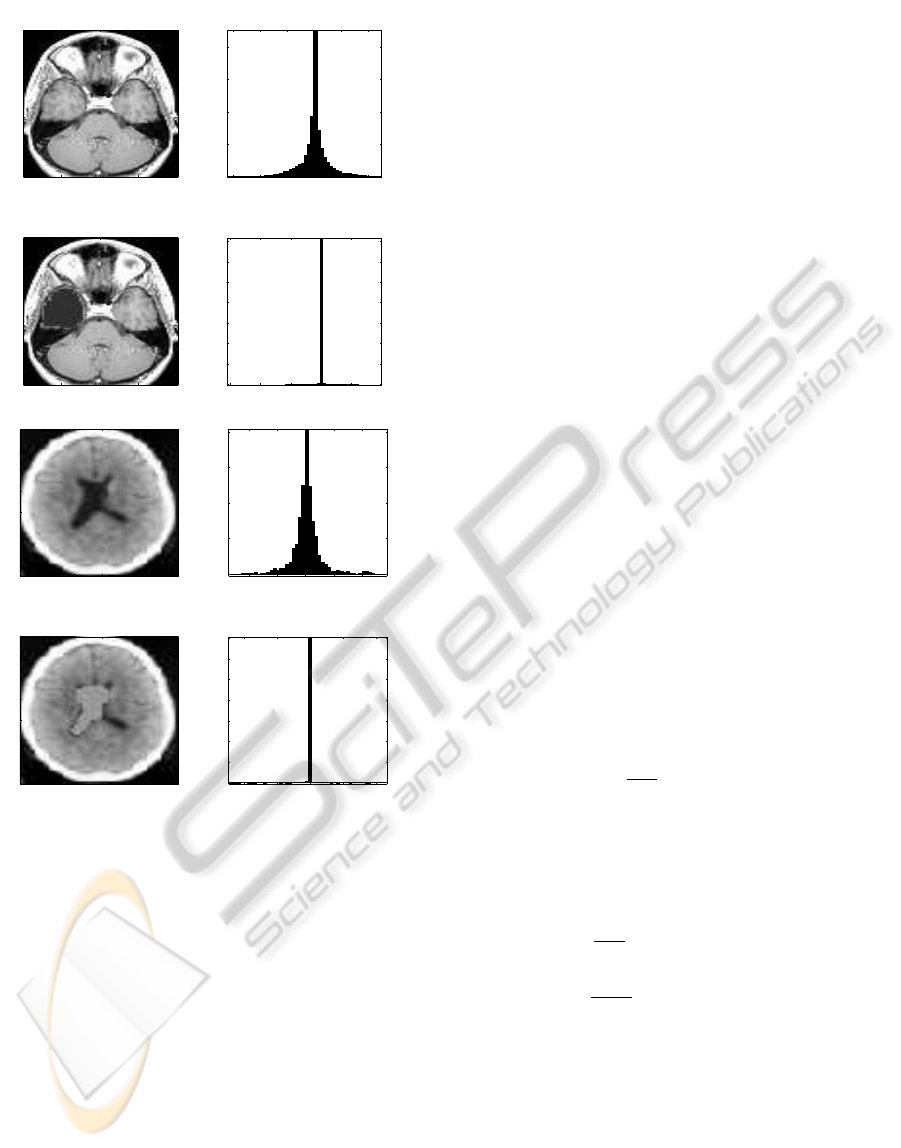
difference will be. Figure 1 shows a few examples
of histograms of the neighbourhood features Dz from
real images, where the sparsity is entirely the con-
sequence of the local smoothness. Additionally, we
also show the histograms of the new neighbourhood
features Df that includes the additional similarity in-
formation. We see the latter is a lot sparser than the
former.
Then we can formulate the i-th feature in a vec-
tor form, with the aid of the i-th row of this matrix
(denoted D
i
) as the following:
f
i
−
1
#
∑
j∈# neighb(i)
f
j
=
N
∑
j=1
d
ij
f
j
= D
i
f (2)
Since our task is to encode the sparse property of
signals, therefore this feature is useful: The differ-
ence between a pixel of the difference image f and
the average of its neighbours is close to zero, almost
everywhere except an the edges of the dissimilarity
areas.
Plugging this into the Pearson-MRF density, we
have the following prior, that we refer to as a
similar-
ity prior
:
Pr(z) =
1
Z
Pr(λ,ν)
N
∏
i=1
{(D
i
(z−s))
2
+ λ}
−
1+ν
2
(3)
where Z
Pr(λ,ν)
=
R
dz
∏
N
i=1
{(D
i
(z−s))
2
+ λ}
−
1+ν
2
is
the partition function that makes the whole probabil-
ity density function integrate to one, and this multi-
variate integral does not have an analytic form.
2.3 Pseudo-likelihood Approximation
As in previous work (A. Kab´an and S. AliPitchay,
2011), we employ a pseudo-likelihood approximation
to the partition function Z
p(λ,ν)
. Replacing the ap-
proximation using the extra information into (3), we
obtain the following approximate image model:
Pr(z|λ,ν) ≈
N
∏
i=1
Γ
1+ν
2
λ
ν/2
{(D
i
(z−s))
2
+ λ}
−
1+ν
2
Γ(
ν
2
)
√
π
(4)
ICPRAM 2012 - International Conference on Pattern Recognition Applications and Methods
124
MRI data 2
20 40 60 80
20
40
60
80
100
−0.6 −0.4 −0.2 0 0.2 0.4
0
500
1000
1500
2000
Histogram of Dz
Lighting change
20 40 60 80
20
40
60
80
100
−0.6 −0.4 −0.2 0 0.2 0.4
0
1000
2000
3000
4000
5000
6000
7000
Histogram of Df
MRI data 1
10 20 30 40 50
10
20
30
40
50
60
70
−0.2 −0.1 0 0.1 0.2
0
200
400
600
800
Histogram of Dz
Lighting change
10 20 30 40 50
10
20
30
40
50
60
70
−0.2 −0.1 0 0.1 0.2
0
500
1000
1500
2000
2500
3000
3500
Histogram of Df
Figure 1: Example histograms of the distribution of neigh-
bourhood features D
i
z, and D
i
f where i=1,...,N from a MRI
real data.
We shall employ this to infer z simultaneously
with estimating our hyper-parameters λ, ν and σ.
2.4 Joint Model
The entire model is the joint model of the observa-
tions y and the unknowns z.
Pr(y,z, f|W,σ
2
,λ,ν)
= Pr(y|z,W,σ
2
)Pr(z|f,λ,ν) (5)
where the first factor is the observation model and the
second factor is the image prior model and its free
parameters λ and ν.
3 MAP ESTIMATION
We will employ the joint probability (5) as the objec-
tive to be maximised. Maximising this w.r.t. z is also
equivalent to finding the most probable image ˆz, i.e.
the maximum a posteriori (MAP) estimate, since (5)
is proportional to the posterior Pr(z|y).
ˆ
z = argmin
z
{−log[Pr(y|z)] −log[Pr(z)]} (6)
Namely, the most probable high resolution signal is
the one for which the negative log of the joint prob-
ability model takes its minimum value. Hence, our
problem can be solved through minimisation. The ex-
pression for the negative log of the joint probability
model will then be defined as our minimisation ob-
jective and also called as the error-objective. It can be
written as:
Obj(z,σ
2
,λ, ν) = −log[Pr(y|z,σ
2
)] −log[Pr(z|f, λ, ν)]
(7)
Equation (7) may be decomposed into two terms: the
first one that contains all the entries that involve z and
the second one contains the terms that do not — i.e.
Obj(z,σ
2
,λ,ν)=Obj
z
(z) + Obj
(λ,ν)
(λ,ν).
3.1 Estimating the most Probable z
The observation model is also called the likelihood
model because it expresses how likely it is that a given
z produced the observed y through the transformation
W. Hence we have for the first term in (5):
Pr(y|z) ∝ exp
−
1
2σ
2
(y−Wz)
T
(y−Wz)
(8)
By plugging in the term for the observation model and
the prior into (7), we obtain the objective function.
The terms of the objective (7) that depend on z are the
following:
Obj
z
(z) =
1
2σ
2
(y−Wz)
2
+
ν+ 1
2
N
∑
i=1
log{(D
i
(z−s))
2
+ λ} (9)
The most probable estimate is the ˆz that has the high-
est probability in the model. It is equivalently the one
that achieves the lowest error. Recap, our model has
two factors which depend on the likelihood or also
known as the observation model, and the image prior
that assists the signal recovery. Thus, our error mod-
els both the
mismatch
of the predicted model Wz
with the observed data y and
determinant
for allow-
ing the free parameters to control the smoothness and
the edges encoded in the prior.
SINGLE-FRAME SIGNAL RECOVERY USING A SIMILARITY-PRIOR BASED ON PEARSON TYPE VII MRF
125

The objective is differentiable; therefore any non-
linear optimiser could be practical to optimise the
term (9) w.r.t. z. The gradient of the negative log
likelihood term is given by:
∇(z)Obj
z
=
1
σ
2
W
′
(Wz−y)+
(ν+ 1)
N
∑
i=1
D
T
i
D
i
(z−s)
(D
i
(z−s))
2
+ λ
(10)
3.2 Estimation of σ
2
, λ and ν
Writing out the terms in (7) that depend on σ
2
, we
obtain a closed form for estimating the σ
2
.
σ
2
=
1
M
M
∑
i=1
(y
i
−W
i
z)
2
!
(11)
Terms that depend on λ and ν are given by:
Obj
(λ,ν)
= N logΓ
1+ ν
2
−NlogΓ
ν
2
+
Nν
2
logλ
−
1+ ν
2
N
∑
i=1
log((D
i
(z−s))
2
+ λ) (12)
Both of these hyperparameters need to be positive val-
ued. To ensure our estimates are actually positive, we
parameterise the log probability objective (12) such as
to optimise for the +/- square root of these parameters.
Taking derivatives w.r.t
√
λ and
√
ν, we obtain:
dlog p(z)
d
√
λ
=
N
∑
i=1
ν(D
i
(z−s))
2
−λ
((D
i
(z−s))
2
+ λ)
√
λ
(13)
dlog p(z)
d
√
ν
=
h
N logλ −
N
∑
i=1
log((D
i
(z−s))
2
+ λ)
+ Nψ
1+ ν
2
−Nψ
ν
2
i
√
ν (14)
where ψ(.) is the digamma function. The zeros of these
functions give us the estimates of ±
√
λ and ±
√
ν. Al-
though there is no closed-form solution, these can be ob-
tained numerically using any unconstrained non-linear
optimisation method
1
, which requires the gradient vec-
tor of the objectives.
3.3 Recovery Algorithm
Our algorithm that implements the equations given in
the previous section is given in Algorithm 1. Note that at
each iteration of the algorithm, two smaller gradient de-
scent problems have to be solved; namely one for λ,
1
We made use of the efficient implementation available
from http://www.kyb.tuebingen.mpg.de/bs/people/carl/
code/minimize/
Algorithm 1: Recovery algorithm.
1: Initialise the estimates z
2: iterate until convergence: do
3: estimate σ
2
using (11)
4: iteratively update λ and ν in turn using defini-
ton
5: (13) and (14), with the current estimate z.
6: iterate to update z using (10)
7: end
ν and one for z. However, experiment suggests that it is
not necessary to estimate the minimum with high accu-
racy. We notice that the inner loops do not require the
entire convergence. It is sufficient to increase but not
necessarily minimise the objective at each intermediate
step.
4 EXPERIMENTS AND
DISCUSSION
We design our experiments for both CS and SR-type W
and we compare with the previous works in (A. Kab´an
and S. AliPitchay, 2011). We devise two hypotheses
to investigate the role of the new prior and we test those
using synthetic 1D and 2D signals and real MRI signals.
Our hypotheses are the following:
• The quality of the recovered signal using the addi-
tional information is no worse than the one without
the extra information provided that the extra infor-
mation is useful. This is when the number of zero
entries in the new form of the neighbourhood fea-
ture, i.e Df is larger than the number of zero entries
in Dz, that is the generic feature that has not been
given the extra similarity information.
• The fewer the edges in f (that is, the non-zeros in
Df), the fewer measurements are sufficient for en-
abling a successful recovery.
Before we proceed with the experiments, we should
mention the construction of the measurement matrix W.
We study two different types: CS-type W is a random
Gaussian matrix (M ×N) with iid entries. The SR-type
W is a deterministic transformation that blurs and down-
samples the image
2
.
4.1 Illustrative 1D Experiments
In this section, we implement our recovery algorithm
on the 1D data, derived from a spike signal
3
of size
2
Code to generate SR-type matrices can be found from
http://www.robots.ox.ac.uk/∼elle/SRcode/ index.html
3
Data taken from http://people.ee.duke.edu/∼lcarin/
BCS.html
ICPRAM 2012 - International Conference on Pattern Recognition Applications and Methods
126
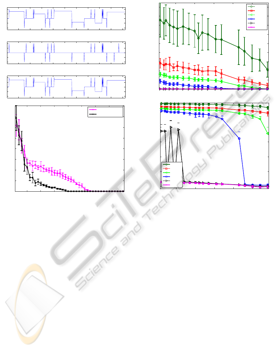
(a)
50 100 150 200 250 300 350 400 450 500
−1
−0.5
0
0.5
1
Original signal
50 100 150 200 250 300 350 400 450 500
−1
−0.5
0
0.5
1
Extra information
50 100 150 200 250 300 350 400 450 500
−1
−0.5
0
0.5
1
PearsonVII similarity prior reconstruction M=190
(b)
50 100 150 200 250 300 350 400
0
0.05
0.1
0.15
0.2
0.25
0.3
0.35
0.4
Number of Measurements
MSE
General prior
Similarity prior
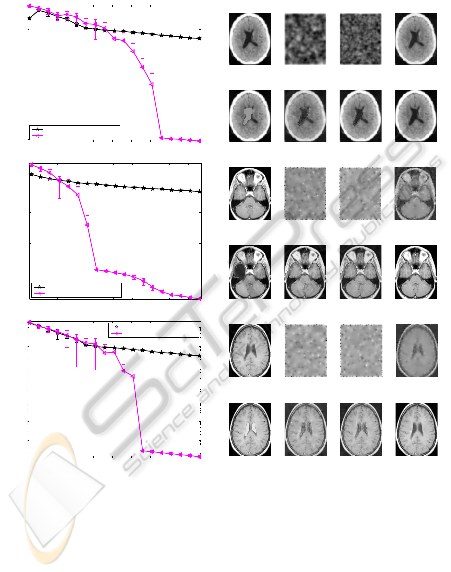
Figure 2: (a) The original spike signal; the extra similarity
information; and an example of recovered signal from 190
measurements. (b) Comparing the MSE performance of 1D
spike signal recovery with and without the extra informa-
tion. The error bars are over 10 independent trials and the
level of noise was σ=8e-5.
512x1 as shown in Figure 2(a). We proceed by plugging
the extra signal into our image prior and varying the
number of measurements using randomly generated
measurement matrices W with i.i.d. Gaussian entries as
in CS. The recovery results are summarised in Figure 2.
We see our enhanced prior is capable to achieve a good
recovery and has a lower mean square error (MSE) than
the one without extra information.
We also examine the MSE performance as a func-
tion of the number of zero entries in the relevant feature
vectors (i.e. Df in our case). Figure 3 shows MSE re-
sults when varying the number of zero entries by con-
structing variations on the signals. We see when the
recovery algorithm received sufficient measurements,
for example when M=250 in Figure 2, the role of the
proposed
similarity prior
gradually reduces. In other
words, this
similarity prior
is
useful
in massively under-
determined problems and provided that the given extra
information has the characteristics described previously.
A widely used alternative way to set hyperparame-
(a)
460 470 480 490 500
0
0.02
0.04
0.06
0.08
0.1
0.12
0.14
0.16
0.18
Number of zero entries in D(z−s)
MSE
M=50
M=100
M=150
M=200
M=250
M=300
(b)
460 470 480 490 500
10
−12
10
−10
10
−8
10
−6
10
−4
10
−2
Number of zero entries in D(z−s)
MSE
M=50
M=100
M=150
M=200
M=250
M=300
Figure 3: (a) Linear scale. (b) Log scale. MSE performance
of 1D spike signal using the extra information. The number
of zero entries in D(z-s) is varied. The error bars represent
one standard error about the mean, from 50 independent tri-
als. The level of noise was σ=8e-5.
ters is cross-validation. It is therefore of interest how
does the automated estimation of the hyper-parameters
of our Pearson type VII based MRF compare to a cross-
validation procedure. Next, we address this by look-
ing at two aspects: MSE performance, and CPU time.
We use the same spike signal for this purpose. For
our comparison, we have chosen 5-folds cross valida-
tion method for estimating the hyper-parameters λ and
ν and the noise variance is assumed to be known for this
method. A sensible search range is pursued to avoid a
long execution time as we are aware that this method
can be extremely time-consuming if the search space is
too large.
Figure 4 shows the MSE performance and the asso-
ciated values for the four levels of noise using the CS-
type W. It is interesting to see that our fully automated
parameter estimation turns out to be superior to 5-folds
cross validation and it has fast convergence and much
lower execution time.
SINGLE-FRAME SIGNAL RECOVERY USING A SIMILARITY-PRIOR BASED ON PEARSON TYPE VII MRF
127
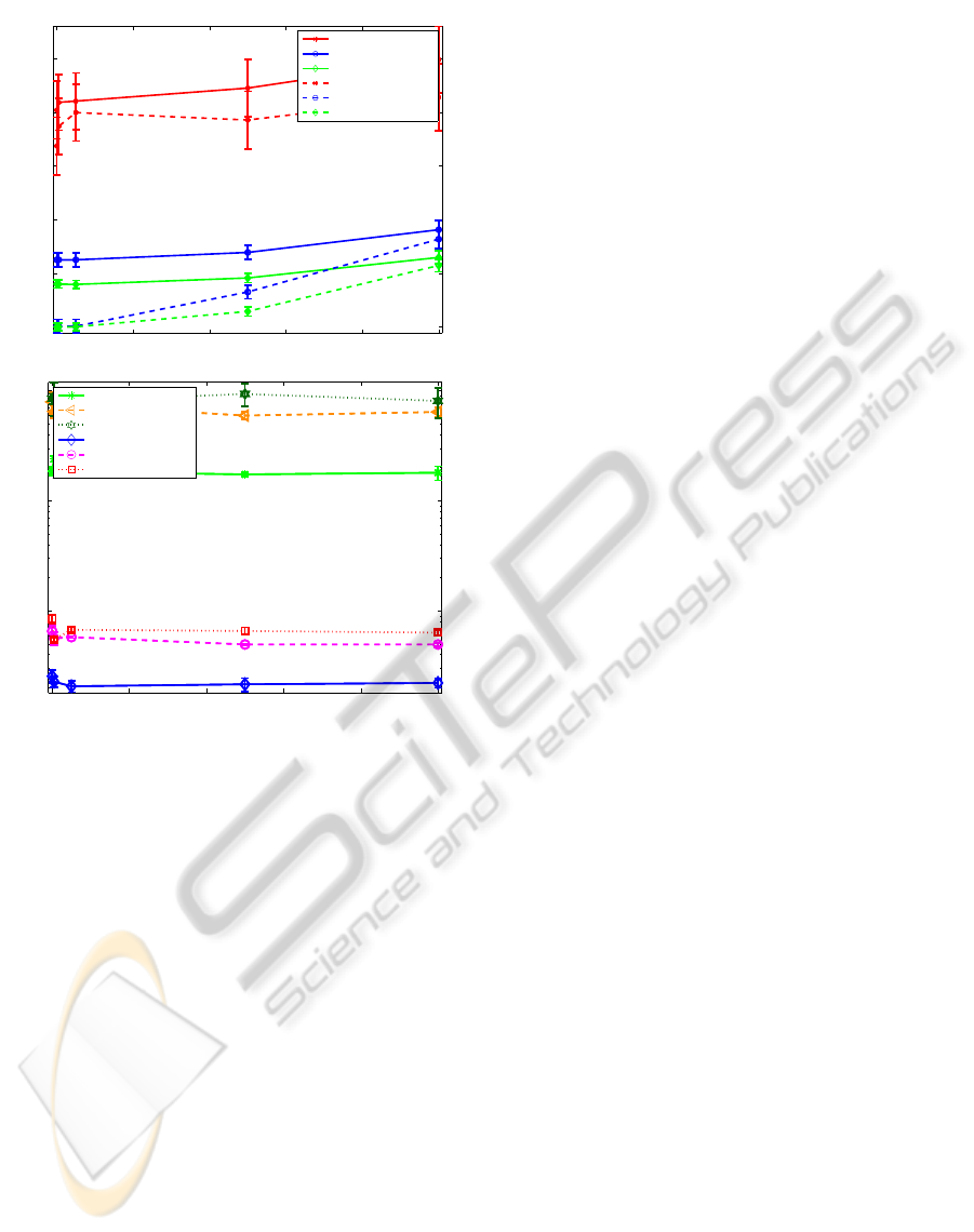
(a)
0 0.2 0.4 0.6 0.8 1
0
0.01
0.02
0.03
0.04
0.05
1D spike signal
Level of noise
MSE
5−folds CV−M=100
5−folds CV−M=240
5−folds CV−M=300
automated−M=100
automated−M=240
automated−M=300
(b)
0 0.2 0.4 0.6 0.8 1
10
2
10
3
10
4
Level of noise
Time(seconds)
5−folds CV−M=100
5−folds CV−M=240
5−folds CV−M=300
automated−M=100
automated−M=240
automated−M=300
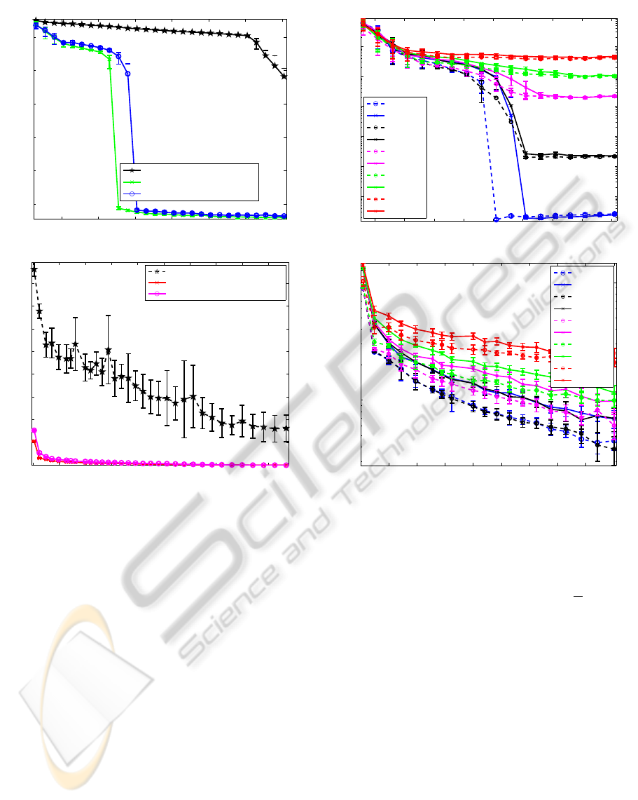
Figure 4: (a) Comparing the MSE performance of the fully
automated Pearson type VII based MRF approach with the
5-folds cross validation, tested with four levels of noise (σ=
0.005, 0.05, 0.5, 1). (b) Cpu time performance against the
same four levels of noise. We see that our automated esti-
mation and recovery is significantly faster than the 5-folds
cross validation method. The error bars are over 10 repeated
trials for each level of noise. Three sets of measurements
(M=100, 240, 300) have been tested for this accuracy com-
parison.
4.2 2D Experiments
Following the thorough understanding gained in the pre-
vious section about when the extra information is help-
ful on the spike signal test cases, we conducted ex-
periments with both compressive sensing (CS) matrices
where W contains random entries and also the classi-
cal super-resolution matrices where W consists of blur
and down-sampling. In this set of experiments, we con-
sider a motionless scene as the extra information. More
precisely, the extra information that we employ in our
similarity-prior consists of a change in the lighting of
some area in the image.
We start by conducting the recovery algorithm on
a synthetic data of size [50x50]. The noise variance σ
tested in all experiments are set to a smaller range in
order to tally the general noise in real data.
Figures 5 and 6 show examples of vastly under-
determined problems using the extra information for re-
covery in comparison with the previous prior devised
in (A. Kab´an and S. AliPitchay, 2011). The MSE per-
formance results are given in Figure 7, and we see the
MSE drops rapidly with increasing the measurement
size. Figure 8 shows examples of recovered images
from this process. We observe that the quality of the re-
covered image increases rapidly for all 5 levels of noise
tested. This is in contrast with the recovery results from
the general prior, which needs a lot more measurements
to perform well.
From these findings, the degree of similarity of the
available extra information has a significant impact on
the recovery from insufficient measurements. We find
that without informative extra information the recovery
algorithm does not perform well with such few mea-
surements. The recovered signal and the MSE using the
artificial Phantom data in figures 5 and 7 demonstrate
that the fewer the edges in the difference imagef the bet-
ter the recovery, or the smaller the number of measure-
ments needed for good recovery. This result validates
our second hypothesis.
In the remainder of the experiments, we will now
focus on image recovery using real image data of mag-
netic resonance imaging (MRI). We obtained this data
from the Matlab database and we created the additional
similarity information from it by changing the lighting
of an area on the image.
Next we validate our second hypothesis on a variety
of MRI images and its lighting changes. The recovery
results for both types of W are presented in figures 10
and 11. The MSE performance for the CS-type W is
shown in figure 9. Interestingly, we observe that the log
scale in that figure is in more direct correspondence with
our visual perception rather than using the standard lin-
ear scale, and this will be seen by comparison to figures
10 and 11.
We observed that more than 6000 measurements are
required for a good recovery without the extra informa-
tion in this example. However, from these results we
see that our similarity prior achieves high quality recov-
ery from an order of magnitude less measurements. The
recovered images are presented in figures 10 and 11 for
visual comparison. Finally, we also show an example
run of our automated parameter estimation algorithm in
Figure 12 for completeness. As one would expect, the
speed of convergence varies with the difficulty of the
problem.
In closing, we should comment on the possibility of
using other types of extra information for signal recov-
ery. Throughout this paper we exploited the similarity
created by a lighting change. Depending on the appli-
cation domain, one might consider a small shift or rota-
tion instead. However, we have seen that the key for the
ICPRAM 2012 - International Conference on Pattern Recognition Applications and Methods
128
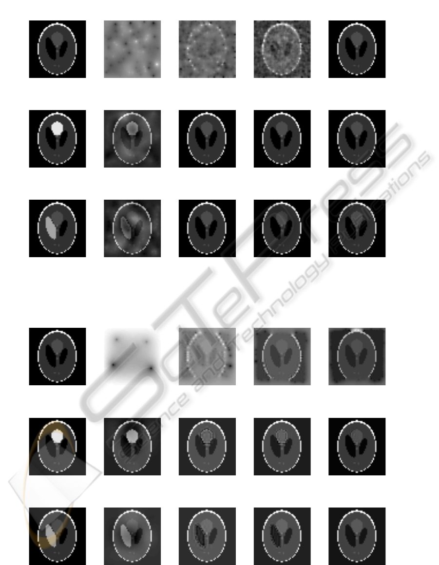
Ground truth a)MSE=1e−001
b)MSE=4e−002
d)MSE=2e−002 e)MSE=6e−012
Sample image recovery without extra information.
Extra info. a)MSE=1e−002
b)MSE=6e−013
d)MSE=3e−013 e)MSE=2e−013
Sample image recovery using extra information of lighting change 1.
Extra info. a)MSE=2e−002
c)MSE=4e−013
d)MSE=3e−013 e)MSE=3e−013
Sample image recovery using extra information of lighting change 2.
Figure 5: Example recovery of 2D synthetic data of size [50x50] in the case of using SR-type W, and given two slightly
different light changes as extra similarity information. The number of measurements (M) are: a) M=60, b) 460, c) 510, d)
960, e) 1310. The additive noise level was σ=8e-5.
Ground truth a)MSE=9e−002
b)MSE=4e−002
d)MSE=2e−002 e)MSE=1e−002
Sample image recovery without extra information.
Extra info. a)MSE=1e−002
b)MSE=8e−004
c)MSE=5e−004 d)MSE=4e−005
Sample image recovery using extra information of lighting change 1.
Extra info. a)MSE=1e−002
b)MSE=1e−003
c)MSE=7e−004 d)MSE=2e−005
Sample image recovery using extra information of lighting change 2.
Figure 6: Example recovery of 2D synthetic data of size [50x50] in the case of using SR-type W, and given two slightly
different light changes as extra similarity information. The number of measurements (M) are: a) M=9, b) 441, c) 784, d)
1296, e) 1849. The additive noise level was σ=8e-7.
SINGLE-FRAME SIGNAL RECOVERY USING A SIMILARITY-PRIOR BASED ON PEARSON TYPE VII MRF
129
200 400 600 800 1000 1200 1400
10
−12
10
−10
10
−8
10
−6
10
−4
10
−2
Number of Measurements
MSE
CS−type W, σ = 8e−5
Without extra info.
Extra info−Lighting change 1
Extra info−Lighting change 2
0 200 400 600 800 1000 1200 1400 1600 1800
0
0.01
0.02
0.03
0.04
0.05
0.06
0.07
0.08
SR−type W, σ = 8e−5
Number of Measurements
MSE
Without extra info.
Extra info−Lighting change 1
Extra info−Lighting change 2
Figure 7: MSE performance of synthetic data [50x50] in
comparison with the two types of extra information. Here,
both types of W were tested and the noise standard deviation
was σ=8e-5.
extra information to be useful in our similarity prior is
that the difference image must have fewer edges than the
original image. This is not the case with shifts or rota-
tions. Therefore to make such extra information useful
we would need to include an image registration model
into the prior. This is subject to future work.
5 CONCLUSIONS
In this paper, we have formulated and employed a
sim-
ilarity prior
based Pearson type VII Markov Random
Field to include the similarity information between the
scene of interest and a consecutive scene that has a light-
ing change. This prior enables us to recover the high res-
olution scene of interest from fewer measurements than
a general-purpose prior would, and this can be applied,
e.g. in medical imaging applications.
100 200 300 400 500 600 700 800 900
10
−7
10
−6
10
−5
10
−4
10
−3
10
−2
Number of Measurements
MSE
CS−type W
Lighting1−σ
1
Lighting2−σ
1
Lighting1−σ
2
Lighting2−σ
2
Lighting1−σ
3
Lighting2−σ
3
Lighting1−σ
4
Lighting2−σ
4
Lighting1−σ
5
Lighting2−σ
5
100 200 300 400 500 600 700 800 900
10
−3
10
−2
Number of Measurements
MSE
SR−type W
Lighting1−σ
1
Lighting2−σ
1
Lighting1−σ
2
Lighting2−σ
2
Lighting1−σ
3
Lighting2−σ
3
Lighting1−σ
4
Lighting2−σ
4
Lighting1−σ
5
Lighting2−σ
5
Figure 8: Recovery of a 50x50 size image from random
measurements (top) and blurred and down-sampled mea-
surement (bottom). The MSE is shown on log scale against
varying the number of measurements, in 5 different levels
of noise conditions. The noise levels were as follows. Top:
σ ∈ {σ
1
=0.005, σ
2
=0.05, σ
3
=0.5, σ
4
=1, σ
5
=2}; Bottom:
{σ
1
=8e-5, σ
2
=8e-4, σ
3
=8e-3, σ
4
=0.016, σ
4
=0.032} — that
is the previous noise levels were divided by 0.8
√
N to make
the signal-to-noise ratios roughly the same for the two mea-
surement matrix types.
ACKNOWLEDGEMENTS
The first author wishes to thank Universiti Sains Islam
Malaysia (USIM) and the Ministry of Higher Education
of Malaysia (MOHE) for the support and facilities pro-
vided.
ICPRAM 2012 - International Conference on Pattern Recognition Applications and Methods
130
(a)
100 200 300 400 500 600 700 800 900
10
−8
10
−6
10
−4
10
−2
Number of Measurements
MSE
Real data 1−Without extra info.
Real data 1−Extra info.
(b)
100 200 300 400 500 600 700 800 900
10
−8
10
−6
10
−4
10
−2
Number of Measurements
MSE
Real data 2−Without extra info.
Real data 2−Extra info.
(c)
100 200 300 400 500 600 700 800 900
10
−7
10
−6
10
−5
10
−4
10
−3
10
−2
10
−1
Number of Measurements
MSE
Real data 3−Without extra info.
Real data 3−Extra info.
Figure 9: MSE performance of real MRI images of size
(a)[70x57], (b) and (c) [100x80], in comparison with three
types of extra information on the three different sets of data.
CS-type W was used and the noise standard deviation was
σ=8e-5.
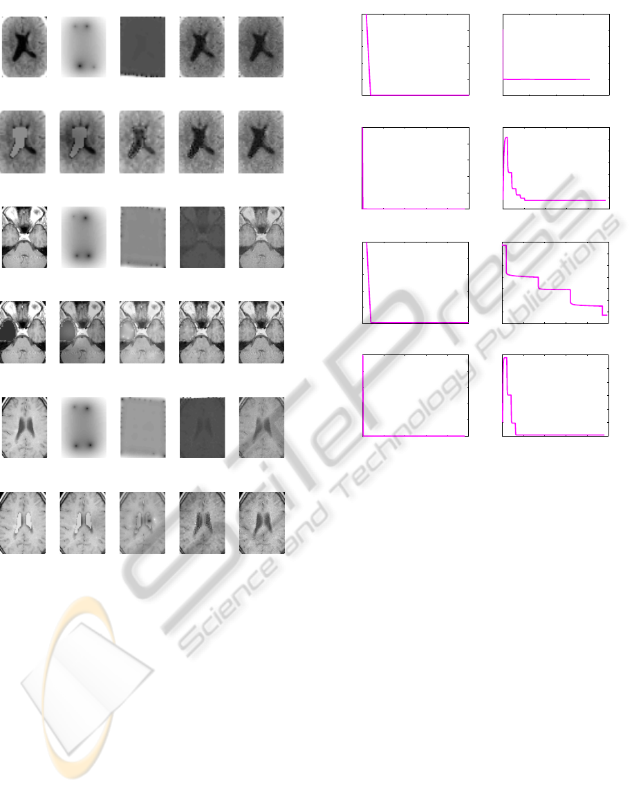
Ground truth a)MSE=1e−002 d)MSE=4e−003 g)MSE=6e−009
Sample image recovery of size [70x57] without extra information.
Extra info. a)MSE=2e−008 d)MSE=5e−009 g)MSE=9e−012
Sample image recovery of size [70x57] using extra information.
Ground truth
c)MSE=7e−003 e)MSE=5e−003
h),MSE=2e−007
Sample image recovery of size [100x80] without extra information.
Extra info.
c)MSE=2e−008 e)MSE=1e−008
h)MSE=3e−011
Sample image recovery of size [100x80] using extra information.
Ground truth
b)MSE=9e−003 e)MSE=5e−003
i)MSE=2e−007
Sample image recovery of size [100x80] without extra information.
Extra info.
b)MSE=4e−008 e)MSE=2e−008
f)MSE=1e−009
Sample image recovery of size [100x80] using extra information.
Figure 10: Examples of MRI image recovery in the case
CS-type W, given a motionless consecutive frame with
some contrast changes. The number of measurements (M)
were: a) M=310, b) 460, c) 560, d) 610, e) 760, f) 1310, g)
3010, h) 5610 i) 7610 and additive noise with σ = 8e-5. The
first two row refers to real data 1, the third row refers to real
data 2 and the fifth row refers to real data 3.
SINGLE-FRAME SIGNAL RECOVERY USING A SIMILARITY-PRIOR BASED ON PEARSON TYPE VII MRF
131
Ground truth a)MSE=51.588
d)MSE=0.100
g)MSE=5e−005 h)MSE=5e−005
Sample image recovery of size [70x57] without extra information.
Partial info. a)MSE=0.00036d)MSE=7e−005 g)MSE=4e−005 h)MSE=4e−005
Sample image recovery of size [70x57] using extra information.
Ground truth a)MSE=139.047
c)MSE=1.273
e)MSE=0.004 i)MSE=0.00371
Sample image recovery of size [100x80] without extra information.
Partial info. a)MSE=0.00071
c)MSE=0.00018
e)MSE=0.00011i)MSE=0.00011
Sample image recovery of size [100x80] using extra information.
Ground truth a)MSE=133.6
b)MSE=3.5
f)MSE=0.0180 i)MSE=0.01799
Sample image recovery of size [100x80] without extra information.
Partial info. a)MSE=8e−004
b)MSE=5e−004
f)MSE=1e−004 i)MSE=1e−004
Sample image recovery of size [100x80] using extra information.
Figure 11: Examples of MRI image recovery in the case
of SR-type W, given a motionless consecutive frame with
some contrast changes. The number of measurements (M)
were: a)M=6, b) 99, c) 154, d) 396, e) 918, f) 1462, g) 1505,
h) 2000, i) 4234. The additive noise is σ=8e-5.
REFERENCES
A. Kab´an and S. AliPitchay (2011). Single-frame image
recovery using a pearson type vii mrf. In Special issue
of Neurocomputing on Machine Learning for Signal
Processing. accepted.
D. L. Donoho (2006). Compressed sensing. IEEE Trans.
Information Theory, 52(4):1289–1306.
E. Candes, J. Romberg, and T. Tao (2006). Robust
uncertainty principles: Exact signal reconstruction
from highly incomplete frequency information. IEEE
Trans. Information Theory, 52(2):489 509.
H. He and L. P. Kondi (2003). Map based resolution en-
(a)
0 5 10 15 20 25
0
0.02
0.04
0.06
0.08
0.1
Iterations
σ
σ estimates
0 2000 4000 6000 8000
−2
0
2
4
6
8
x 10
7
Iterations
Objective: − log p(y,z)
0 50 100 150 200 250
0
0.01
0.02
0.03
0.04
0.05
Iterations
λ
λ estimates
0 50 100 150 200 250
0
0.1
0.2
0.3
0.4
0.5
0.6
0.7
Iterations
ν
ν estimates
(b)
0 5 10 15 20 25
0
0.02
0.04
0.06
0.08
0.1
Iterations
σ
σ estimates
0 2000 4000 6000 8000 10000
−6
−5
−4
−3
−2
−1
0
1
x 10
4
Iterations
Objective: − log p(y,z)
0 50 100 150 200 250
0
0.1
0.2
0.3
0.4
0.5
Iterations
λ
λ estimates
0 50 100 150 200 250
0.06
0.08
0.1
0.12
0.14
0.16
0.18
Iterations
ν
ν estimates
Figure 12: Example evolution of the hyper-parameter up-
dates (σ, λ, ν) and objective function versus the number
of iterations of the optimisation algorithm while recovering
a 2D signal: (a) from M=460 random measurements; (b)
from a blurred and down-sampled low resolution frame of
M=144. In both experiments, the level of noise was σ=8e-5.
hancement of video sequences using a huber-markov
random field image prior model. In IEEE Conference
of Image Processing, pages 933–936.
H. He and L. P. Kondi (2004). Choice of threshold of the
huber-markov prior in map based video resolution en-
hancement. In IEEE Electrical and Computer Engi-
neering Canadian Conference, volume 2, pages 801–
804.
JCR. Giraldo, JD. Trzasko, S. Leng, CH. McCollough, and
A. Manduca (2010). Non-convex prior image con-
strained compressed sensing (nc-piccs). In Proc. of
SPIE : Physics of Medical Imaging, volume 7622.
L. C. Pickup, D. P. Capel, S. J. Roberts, and A. Zissermann
(2007). Bayesian methods for image super-resolution.
The Computer Journal.
N. Vaswani and W. Lu (2010). Modified-cs: Modify-
ing compressive sensing for problems with partially
known support. IEEE Trans. on Signal Processing,
58(9).
RC. Hardie and KJ. Barnard (1997). Joint map registra-
tion and high-resolution image estimation using a se-
ICPRAM 2012 - International Conference on Pattern Recognition Applications and Methods
132

quence of undersampled images. IEEE Trans. Image
Processing, 6(12):621–633.
R. G. Baraniuk, V. Cevher, M. F. Duarte, and C. Hegde
(2010). Model-based compressive sensing sensing.
IEEE Trans. Information Theory, 56:1982–2001.
S. Ji, Y. Xue, and L. Carin (2008). Bayesian compressive
sensing. IEEE Trans. Signal Processing, 56(6):2346–
2356.
W. Lu and N. Vaswani (2011). Regularized modified bpdn
for noisy sparse reconstruction with partial erroneous
support and signal value knowledge. IEEE Trans. on
Signal Processing, To Appear.
SINGLE-FRAME SIGNAL RECOVERY USING A SIMILARITY-PRIOR BASED ON PEARSON TYPE VII MRF
133
