UNDERSTANDING TOA AND TDOA NETWORK CALIBRATION
USING FAR FIELD APPROXIMATION AS INITIAL ESTIMATE
Yubin Kuang, Erik Ask, Simon Burgess and Kalle
˚
Astr¨om
Centre for Mathematical Sciences, Lund University, Lund, Sweden
Keywords:
TOA, TDOA, Calibration, Sensor networks, Self-localization.
Abstract:
This paper presents a study of the so called far field approximation to the problem of determining both the
direction to a number of transmittors and the relative motion of a single antenna using relative distance mea-
surements. The same problem is present in calibration of microphone and wifi-transmittor arrays. In the far
field approximation we assume that the relative motion of the antenna is small in comparison to the distances
to the base stations. The problem can be solved uniquely with at least three motions of the antenna and at
least six real or virtual transmittors. The failure modes of the problem is determined to be (i) when the an-
tenna motion is planar or (ii) when the transmittor directions lie on a cone. We also study to what extent the
solution can be obtained in these degenerate configurations. The solution algorithm for the minimal case can
be extended to the overdetermined case in a straightforward manner. We also implement and test algorithms
for non-linear optimization of the residuals. In experiments we explore how sensitive the calibration is with
respect to different degrees of far field approximations of the transmittors and with respect to noise in the data.
1 INTRODUCTION
Navigation covers a broad application area ranging
from traditional needs in the terrestrial, aerial and
naval transport sectors to personal objectives of find-
ing your way to school if you are visually impaired,
to the nearest fire exit in case of an emergency, or to
specific goods in your local supermarket. Many po-
tential applications are however presently hindered by
performance limitations of existing positioning tech-
niques and navigation systems.
Radio based positioning rely on either signal
strength, direction of arrival (DOA) or time-based in-
formation such as time of arrival (TOA) or time dif-
ferences of arrival (TDOA), or a combination thereof.
The identical mathematical problem occurs also
in microphone arrays for audio sensing. Using mul-
tiple microphones it is possible to locate a particu-
lar sound-source and using beamforming to enhance
sound quality of the speaker.
Although TOA and TDOA problems have been
studied extensively in the literature in the form of lo-
calization of e.g. a sound source using a calibrated
detector array, the problem of calibration of a sen-
sor array using only measurement, i.e. the initializa-
tion problem for sensor network calibration, has re-
ceived much less attention. One technique used for
sensor network calibration is to manually measure the
inter-distance between pairs of microphones and use
multi-dimensional scaling to compute microphone lo-
cations, (Birchfield and Subramanya, 2005). Another
option is to use GPS, (Niculescu and Nath, 2001), or
to use additional transmittors (radio or audio), close to
each receiver, (Elnahrawy et al., 2004; Raykar et al.,
2005; Sallai et al., 2004). Sensor network calibra-
tion is treated in (Biswas and Thrun, 2004). In (Chen
et al., 2002) it is shown how to estimate additional mi-
crophones, once an initial estimate of the position of
some microphones are known. In (Thrun, 2005) the
far field approximation is used to initialize the cali-
bration of sensor networks. However the experiments
and theory was only tested for the planar case and
no study of the failure modes were given. Initializa-
tion of TOA networks has been studied in (Stew´enius,
2005), where solutions to the minimal case of three
transmittors and three receivers in the plane is given.
The minimal case in 3D is determined to be four re-
ceivers and six transmittors for TOA, but this is not
solved. Initialization of TDOA networks is studied
in (Pollefeys and Nister, 2008), where solutions were
give to two non-minimal cases of ten transmittors and
five receivers, whereas the minimal solution for far
field approximation in this paper are six transmittors
and four receivers.
590
Kuang Y., Ask E., Burgess S. and Åström K. (2012).
UNDERSTANDING TOA AND TDOA NETWORK CALIBRATION USING FAR FIELD APPROXIMATION AS INITIAL ESTIMATE.
In Proceedings of the 1st International Conference on Pattern Recognition Applications and Methods, pages 590-596
DOI: 10.5220/0003793305900596
Copyright
c
 SciTePress

In this paper we study far field approximation as
an initialization to the calibration problem. We use a
similar factorization as (Thrun, 2005) but in three di-
mensions, and show that far field approximation is at
least four measurement positions, i.e. three motions,
and measurements to at least six real or virtual trans-
mittors. In this paper we describe the failure modes of
the algorithm and show what can be done when such
configurations are present. We further propose two
optimization strategies for more thorough calibration
and evaluate them in regards to accuracy and conver-
gence rate. Several test cases are simulated in which
we validate far field approximation, accuracy of the
proposed algorithms, optimization schemes and per-
formance under noisy measurements.
2 DETERMINING POSE
In the following treatment, we make no difference be-
tween real and virtual transmittors or base stations.
Assume that the base station is stationary at posi-
tion b =

b
x
b
y
b
z

and that the antenna is at po-
sition z =

z
x
z
y
z
z

. By measuring the signal
with known base band frequency one obtains a com-
plex constant, whos phase depends on the distance
d = |b − z| between the antenna and the base station.
By tracking the phase during small relative mo-
tions of the antenna, it is feasible to determine the
relative distance d
rel
(t) = d(t) +
˜
C, where
˜
C is an un-
known constant for each base station. This is the so
called TDOA setup. Furthermore if during measure-
ments the relative motion is small in comparison with
the distance d between the antenna z and the base sta-
tion b it is reasonable to approximate the distance d =
|b−z| ≈ |b−z
0
|+(z−z
0
)
T
n= z
T
n+(|b− z
0
| − z
T
0
n)
|
{z }
¯
C
.
Here z
0
is the initial position of the antenna and n
is the direction from the base station towards the an-
tenna, now assumed to be constant with unit length.
By settingC =
˜
C+
¯
C one obtains the far field approx-
imation
d
rel
(n,z) ≈ z
T
n+C.
In this paper we are interested in the following far
field time difference of arrival (FFTDOA) type prob-
lem that arise from this approximate relative distance
measurement.
Problem 1. Given measurements D
i, j
, i =
1,. .. ,m and j = 1,... ,k from the antenna at m
different positions to k base stations, determine both
the positions z
1
,...,z
m
of the antenna during the
relative motion and the directions n
1
...n
k
from the
base stations so that
D
i, j
= z
T
i
n
j
−C
j
,
||n
j
||
2
= 1
where C
j
is a constant distance offset for each base
station.
Lemma 1. A problem with m measurements to k base
stations with unknown constant C
j
can without loss
of generality be converted to a problem with m − 1
measurements to k base stations with known constant.
Proof. Note that because of the unknown constant C
j
the problem does not change in character by modifi-
cation
¯
D
i, j
= D
i, j
− K
j
. For simplicity we set
¯
D
i, j
=
D
i, j
− D
1, j
. By also setting z
1
=

0 0 0

T
, we get
C
j
= 0. This is equivalent to choosing the origin of
the unknown coordinate system to the first point.
For simplicity we will in the sequel assume that
C
j
= 0 and assume that the one measurement has al-
ready been used to resolve the ambiguity. Denote by
D the matrix after removing that said point. This con-
verts the FFTDOA problem into a FFTOA problem,
i.e.
Problem 2. Given measurements D
i, j
, i =
1,. .., m, j = 1,..., k from the antenna at m dif-
ferent positions to k base stations, determine both the
both the positions z
i
of the antenna during the relative
motion and the direction from the base stations n
j
so
that
D
i, j
= z
T
i
n
j
.
||n
j
||
2
= 1
Lemma 2. The matrix D with elements D
i, j
is of rank
at most 3.
Proof. The measurement equations are D
i, j
= z
T
i
n
j
.
By setting
Z =





z
T
1
z
T
2
.
.
.
z
T
m





and
N =

n
1
n
2
... n
k

we see that D = ZN. Both Z and N have at most rank
3, therfore the same holds for D.
Assuming that k and m are large enough and as-
suming that the motion z
i
and the base stations n
j
are
in general enough constellation the matrix D will have
rank 3. If so it is possible to reconstruct both Z and N
up to an unknown linear transformation. This can be
done using singular value decomposition, D = USV
T
.
UNDERSTANDING TOA AND TDOA NETWORK CALIBRATION USING FAR FIELD APPROXIMATION AS
INITIAL ESTIMATE
591

Even with noisy measurements, the closest rank 3 ap-
proximation in the L
2
norm can be found using the
first 3 columns of U and V. By setting
˜
Z = U
3
and
˜
N = S
3
V
T
3
we get all possible solutions by N = A
˜
N,
with A a general full rank 3× 3 matrix. Changing A
corresponds to rotating, affinely stretching and pos-
sibly mirroring the coordinate system. The true re-
construction also fulfills n
T
j
n
j
= 1, which gives con-
straints on A of type
n
T
j
A
T
An
j
= 1,
which after substitution B = A
T
A becomes linear
n
T
j
Bn
j
= 1
in the unknown elements of B. Since symmetric
3× 3 matrices have 6 degrees of freedom we need at
least 6 base stations to determine the matrix uniquely.
Once B has been determined A can be determined by
Cholesky factorization. This gives the transformation
A up to an unknown rotation and possible mirroring
of the coordinate system. We summarize the above in
the following theorem.
Theorem 1. The minimal case for reconstructing m
positions z
i
and k orientations n
j
from relative dis-
tance measurements D
i, j
as formulated in Problem 2
is m = 4 and k = 6.
Accordingly, we have the following algorithm for
the minimal case of the problem:
Algorithm 1.
Given the measurement matrix D of size 4× 6.
1. Set
¯
D
i, j
= D
i, j
− D
1, j
2. Remove the first row of
¯
D
3. Calculate a singular value decomposition
¯
D =
USV
T
.
4. Set
˜
Z to first 3 columns of U and
˜
N to first three
columns of SV
T
.
5. Solve for the six unknowns in the symmetric ma-
trix B using the 6 linear constraints ˜n
T
j
B˜n
j
= 1.
6. Calculate A by Cholesky factorization of B, so that
A
T
A = B.
7. Transform motion according to Z =
˜
ZA
−1
and
structure according to N = A
˜
N.
Note that using minimal information m = 4 and
k = 6 results in estimates that fulfill the measurements
exactly (up to machine precision) evenif the measure-
ments are disturbed by noise.
2.1 Failure Modes of the Algorithm
It is interesting and enlightening to know the failure
modes of the algorithm. This is captured by the fol-
lowing theorem.
Theorem 2. The minimal case for reconstructing m
orientations n
j
and k positions z
i
from relative dis-
tance measurements D
i, j
as formulated in Problem
2 is for m = 4 and k = 6. As long as the orien-
tations n
j
do not lie on a common quadratic cone
n
T
j
Ωn
j
= 0 and the measurement positions z
i
do not
lie on a plane, there will not be more than one solu-
tion to the problem of determining both structure n
j
and motion z
i
up to an unknown translation, orienta-
tion and reflection of the coordinate system.
Proof. The algorithm can fail if the measurement ma-
trix D has rank 2 or lower. This could e.g. happen if
either all measurement positions z
i
lie in a plane or if
all directions n
j
lie in a plane (or both). The algorithm
can also fail if there are two solutions to the matrix B
in n
T
j
Bn
j
= 1. But then the difference Ω = B
1
− B
of these two solutions is a three by three matrix for
which
n
T
j
Ωn
j
= 0,
which in turn implies that the directions n
j
lie on a
common conic as represented by the matrix Ω.
Yet another type of failure mode of the algorithm
is if the data is corrupted by noise or far field approxi-
mation is not vaild, so that the matrix B obtained is not
positive definite. Then the algorithms fails because
there is no Cholesky factorization of B into A
T
A. If B
is unique, there are no real solution to the problem in
this case.
2.2 Analysis of Failure Modes
If the rank of the matrix D is 2, this could be because
the points z
i
lie on a plane or that n
j
lie on a plane.
In this case of coplanar z
i
it is still possible to esti-
mate the planar coordinates Z = U
2
A and N = AS
2
V
T
2
up to an unknown2×2 matrix A representinga choice
of affine coordinate system. Here we do get inequality
constraints that




A

n
j,x
n
j,y





≤ 1.
Each such A is a potential solution. It is possible to
extend with a third coordinate in the normal direction
according to
n
j,z
= ±
q
1− n
2
j,x
− n
2
j,y
.
Another possibility is that the directions n
j
lie on
a plane. In this case it is possible to reconstruct two
of the coordinates for both the positions z
i
and the
directions n
j
. Since the normals are assumed to lie
in a plane, we can exploit the equality constraints
n
T
j
A
T
An
j
= 1 similar to the rank 3 case. In this par-
ticular case we only need three directions n
j
, i.e. the
ICPRAM 2012 - International Conference on Pattern Recognition Applications and Methods
592

minimal case is for m = 3 and k = 3. This gives the
full reconstruction of both points and directions up to
an unknown choice of Euclidean coordinate system
and unknown choice of z-coordinate for the points z
i
.
If the rank is 1, this could be because the direc-
tions are parallel. In this case. Similar to the discus-
sions above we can obtain one of the coordinates of
the positions z
i
, but this is trivial since the measure-
ments D
i, j
are such coordinates by definition.
If the rank is 1 because the points lie on a line,
we obtain a one-parameter family of reconstructions
based on Z = U
1
a and N = aS
1
V
T
1
, where a is an
unknown constant that has to fulfill a ≤ 1/l, where
l = max
j
|S
1
V
1, j
|. For each such a it is possible to ex-
tend the directions n
j
so that they have length one, but
there are several such choices.
2.3 Overdetermined Cases
When more measurements are available than the min-
imal case discussed in the previous section, we need
to solve an overdetermined system in least-square
sense or with robust error measures e.g. L
1
-norm.
Here we focus on the following least-square formu-
lation for the pose problem:
Problem 3. Given measurements D
i, j
, i =
1,. .. , m and j = 1,. ..,k from the antenna at m
different positions to k base stations, determine both
the relative motion of the antenna z
i
and the direction
to the base stations n
j
so that
min
Z,N
||D− Z
T
N||
2
Frob
(1)
s.t. ||n
j
||
2
= 1, j = 1,... ,k.
where ||.||
Frob
denotes the Frobenius norm.
For the over-determined cases, that is m > 4 and
k ≥ 6 or m ≥ 4 and k > 6, it is possible to modify
Algorithm 1 to obtain an efficient but not necessarily
optimal algorithm that finds a reconstruction that fits
the data quite good using the following three mod-
ifications (i) the best rank 3 approximation can still
be found in step 4-5 using the singular value decom-
position, (ii) the estimate of B in step 6 can be per-
formed in a least squares sense and (iii) re-normalize
the columns of N to length 1. This results in a recon-
struction that differs from the measurements, but both
steps are relatively robust to noise. The problem of
B not being positive semi-definite can be attacked by
non-linear optimization. Here we try to optimize A so
that
∑
k
j=1
(n
T
j
A
T
An
j
− 1)
2
is minimized. This can be
achieved e.g. by initializing with A = I and then using
non-linear optimization of the error function.
Clearly, we lose any guarantee on the optimality
of the solution when we enforce the constraints as in
step (iii). However, the solution can serve as a good
initialization for subsequent optimization algorithms
we present in this section. We discuss how to use al-
ternating optimization and Levenberg-Marquardt al-
gorithm (LMA) to obtain better solution. The first
algorithm starts with an initial feasible solution for
Z and N, and then it alternates between optimizing
Z given N and vice versa. The latter is essentially
a method combining Gauss-Newton algorithm and a
gradient descent that improve the solution locally. For
both methods, we need to treat the constraints on the
direction vectors properly to ensure convergence.
2.3.1 Alternating Optimization
In order to find the local minima of Problem 3, we
can use a coordinate descent scheme. Specifically, we
would like to iteratively optimize the cost function in
Problem 3 with respect to Z given N, and then find
the optimal feasible N with fixed Z. If we initialize
N such that it satisfies the norm constraints, we can
easily see that the alternating procedure is converging
(Algorithm 2).
Algorithm 2.
Given the measurement matrix D with m > 4 and k ≥
6 or m ≥ 4 and k > 6,
1. Construct
¯
D and initialize Z and N as in Algo-
rithm 1
2. Fix N , find optimal Z
3. Fix Z, solve the constrained minimization for each
n
j
, j = 1,...,k
4. Repeat (2) and (3) until convergence or predefined
number of iterations is reached
To enable the alternating optimization, we need
to solve two separate optimization problems. The
first one is to find the optimal Z given N. This is
the classic least squares problem and is known to be
convex and can be solved efficiently. On the other
hand, solving for optimal n
j
given Z is not always
convex due to the additional constraints on the n
j
’s.
In this case, we seek the local minima for each n
j
as a constrained minimization problem. We solve the
small constrained problems (3 variables each) inde-
pendently with interior point method. Alternatively,
we can solve the constrained optimization as solv-
ing polynomial equations. This can be related to the
fact that for a given Z, level sets of the cost function
with respect to n
j
are surfaces of a ellipsoid in R
3
(the centers are in this case the solution from singu-
lar value decomposition). The norm 1 constraints on
n
j
geometrically means that the feasible solutions lie
on the unit sphere centered at origin. Therefore, the
optimal solution of n
j
is one of the points that the
UNDERSTANDING TOA AND TDOA NETWORK CALIBRATION USING FAR FIELD APPROXIMATION AS
INITIAL ESTIMATE
593

ellipsoid is tangent to the unit sphere, which can be
found by solving polynomial equations. While there
could exist multiple solutions, we can choose the one
with minimum euclidean distances to the center of
the ellipsoid. Unlike interior point solver, we always
find the global optimum. However, in practice, we
found that in the alternating procedure, interior point
method and polynomial solving give similar perfor-
mance.
2.3.2 Levenberg-Marquardt Algorithm
It is well-known that alternating optimization as a co-
ordinate descent scheme convergesslowly in practice.
Alternatively, we can solve the minimization problem
by iteratively finding the best descent direction for N
and Z simultaneously. The difficulty here is again
the constraints on the direction vectors n
j
. The key
idea here is to re-parameterize the orientation vec-
tors. Given a direction vector n having unit length,
any direction vectors can be represented by n·exp(S),
where S is a 3×3 skew-symmetric matrix. This is due
to the fact that the exponential map of any such matrix
is a rotation matrix. In this case, if we use the (cur-
rent) orientation n as axis direction, any local change
of the orientation on the sphere can be easily parame-
terized via the exponential map. Therefore, the gradi-
ent of D
ij
with respect to n
j
can be expressed without
any constraints. We can then construct the Jacobian
for the Levenberg-Marquardt algorithm to compute
the optimal descent direction. In the following, we
use y to denote the vector formed by stacking vari-
ables in Z and N,
¯
d is the vectorized version of
¯
D
based on the ordering of g.
Algorithm 3.
Given the measurement matrix D (over-determined),
initialize y and construct
¯
d as in Algorithm 1,
1. Compute the Jacobian of
¯
d with respect to y, J =
(
∂
¯
D
11
∂y
,...,
∂
¯
D
ij
∂y
,...,
∂
¯
D
(m−1)k
∂y
)
2. Calculate ∆y = (J
T
J + λ · diag(J
T
J))
−1
J
T
∆
¯
d,
where ∆
¯
d is the residue and λ a damping factor.
3. y = y + ∆y
4. repeat (1),(2) and (3) until convergence or prede-
fined number of iterations is reached
3 EXPERIMENTAL VALIDATION
In this section, we present comprehensive experimen-
tal results for simulated data. We focus on the per-
formance of the minimal solver, verification of the far
10
2
10
4
10
6
10
−7
10
−6
10
−5
10
−4
10
−3
10
−2
10
−1
10
0
Relative Distance
Error in Position
Farfield Approximation performance
Failure Rate
0
0.05
0.1
0.15
0.2
0.25
0.3
0.35
0.4
0.45
0.5
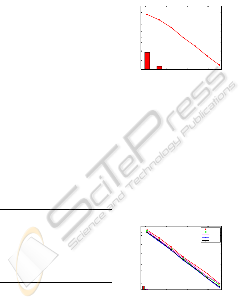
Figure 1: Performance on minimal case solver. Bars show
failure rate (left y-axis) and curve shows the norm in esti-
mated position as a function of distance (right y-axis). Note
that bar height has linear scale.
field approximation as well as the comparisons be-
tween solvers for overdetermined cases.
3.1 Minimal Solver Accuracy
The numerical performance of the algorithm was
evaluated by generating problems where the far field
approximation is true and not degenerate. In essence
this constitutes generating directions n
j
and relative
distance measurements D
i, j
and culling cases where
the three largest singular values of the measurement
matrix aren’t above a threshold or the directions lie
on a conic. The error is then evaluated as the average
norm-difference of the estimated reciever positions.
The reciever positions were selected as the corners of
a tetrahedron with arc-length one. The average error
of 10000 such tests was 6.8· 10
−15
, close to machine
epsilon.
10
2
10
4
10
6
10
−8
10
−7
10
−6
10
−5
10
−4
10
−3
10
−2
10
−1
Relative Distance
Error in Position
Non minimal Solver performance
r4 − s8
r4 − s10
r5 − s10
r6 − s15
r10 − s30
Failure Rate
0
0.05
0.1
0.15
0.2
0.25
0.3
0.35
0.4
0.45
0.5
Figure 2: Performance on non-minimal cases. Bars show
failure rates, line is error as a function of distance in loglog
scale. Size of test-cases are noted in figure with rx-sy de-
noting x recievers and y senders. This plot is best viewed in
color. Note the scale difference to the graph in Figure 1.
ICPRAM 2012 - International Conference on Pattern Recognition Applications and Methods
594

3.2 Far Field Approximation Accuracy
3.2.1 Minimal Case
To evaluate the performance of the assumption that
senders can be viewed as having a single common
direction to receivers, data was generated using 3D
positions for both senders and receivers at different
relative distances in-between receivers and senders
to receivers. The constellation of receivers is again
the tetrahedron and senders are randomly placed on a
sphere surrounding it. A graph showing the error, as
defined in section 3.1, as a function of radius of the
sphere (that is relative distance), as well as the failure
rate of the solver is shown in Figure 1. A failure con-
stitutes a case in which the B matrix in algorithm 1 is
not positive definite. As can be seen this is infrequent
even at small relative distances in when one would
not expect a far field approximation to work. As can
be expected the approximation gets better when the
relative distance increases.
3.2.2 Initialization for Overdetermined Cases
As described in section 2.3 algorithm 1 can with some
modifications be used on overdetermined cases with-
out guarantees on optimality of the solution. In these
situations the solutions serves as an initial guess of
some other optimization method. The additional in-
formation should however give some numerical sta-
bility and it is interesting to evaluate the algorithm for
initial guess estimates in overdetermined cases. To do
this the synthetic dataset is augmented with additional
randomly placed senders and receivers. The four first
receivers are again the tetrahedron and the rest are
randomly uniformly distributed within the unit cube.
Senders are again placed on a sphere around the re-
ceivers. Results for different problem sizes are shown
in Figure 2. One immediately notices that the fail-
ure ratio drops, in many cases to zero. One can also
see that adding more data will (in general) result in
smaller errors, for the cases shown here up to one or-
der of magnitude smaller than a min case.
3.3 Overdetermined Cases
We also investigate the performance of the two
schemes for over-determined cases. In all experi-
ments below, we initialize both the alternating op-
timization and LMA based on the minimal solver
modified for over-determined case. The simulated
data is of a true far field approximation with gaus-
sian white noise, i.e. measurements are simulated as
D
i, j
= z
i
n
j
+ ε
i, j
where ε
i, j
∈ N(0,σ) i.i.d. In Fig-
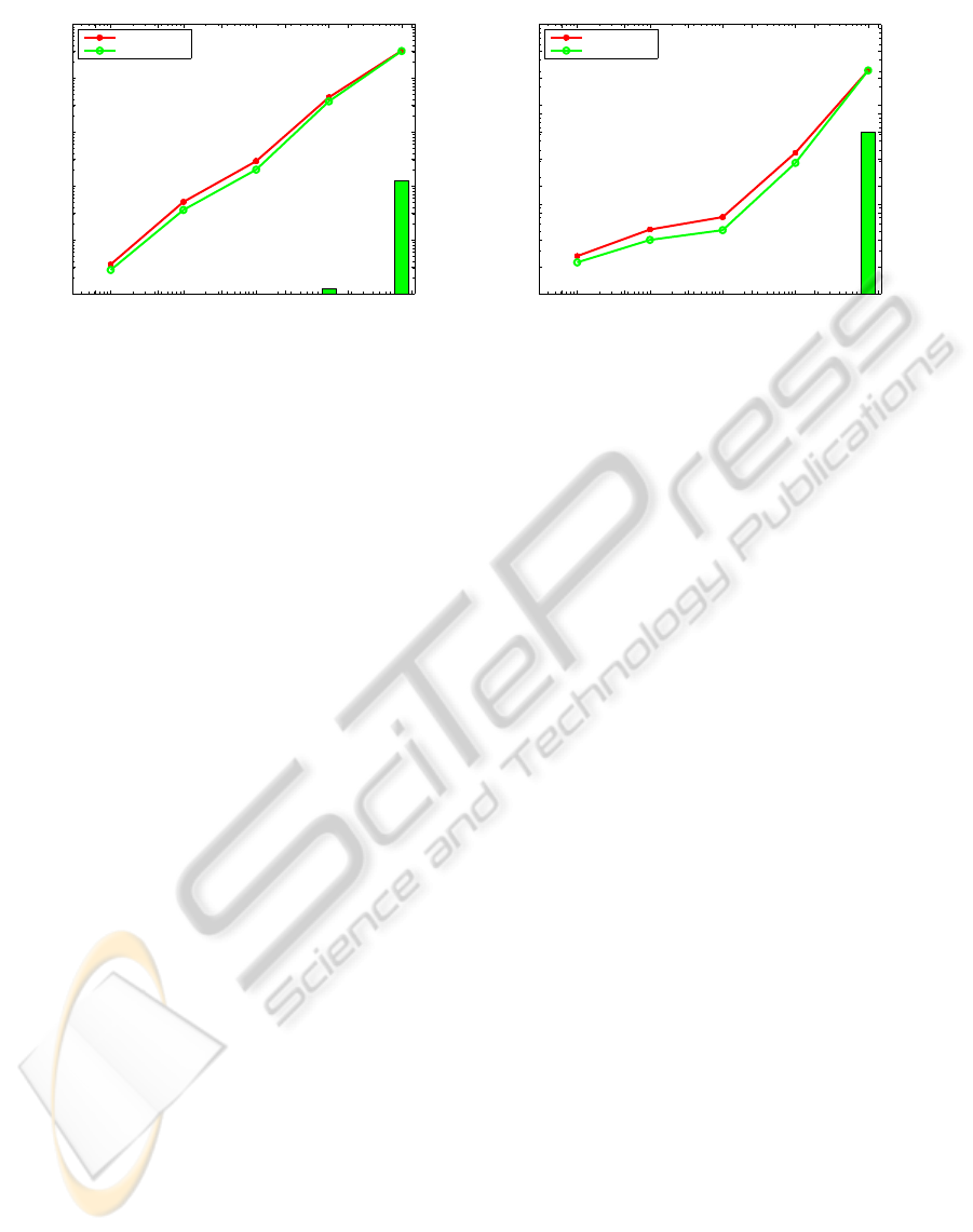
ure 3, we can see that alternating optimization and
0 50 100 150
10
−20
10
−15
10
−10
10
−5
10
0
E−E
min *
AlterOpt
LMA
Figure 3: Convergence of alternating optimization and
LMA on simulated TDOA measurements with gaussian
white noise (σ = 0.1). Here m = 10 and k = 10.
LMA all decrease the reconstruction errors compared
to the minimal solver. On the other hand, from fig-
ure 3, LMA converges much faster than alternating
scheme (20 vs. 150) and obtains relatively lower re-
construction errors. This verifies the superiority of
LMA over coordinate descent. This observation is
consistent over different m and k as well as a variety
of noise levels. Note that here for all the experiments,
we set the damping factor λ to 1.
It it also of interest to view the complete sys-
tem when the measurements D
i, j
does not fulfill the
far field approximation and when disturbed by noise.
The relative distances of the simulated senders and
receivers are set to 10
2
for a mediocre far field ap-
proximation and 10
7
for a good far field approxima-
tion. TDOA measurements D
i, j
are then simulated,
perturbed with gaussian white noise. Figure 4 shows
the results. The pictures show that the initialization
method is fairly good, but in many cases the LMA
brings down the position error. The system is also
fairly robust to noise.
4 CONCLUSIONS
In this paper we study the far field approximation to
the calibration of TDOA and TOA sensor networks.
The far field approximation of the problem results in
a factorization algorithm with constraints. The failure
modes of the algorithm is studied and particular em-
phasis is made on what can be said when any of these
failure conditions are met. The experimental valida-
tion gives a strong indication that a far field approx-
imation is a feasible approach both for getting direct
estimates as well as initial estimates for other solvers.
Even considering that there are cases when the algo-
rithm fails, obtained solutions are good even at small
relative distances. This validation is done on 3D prob-
UNDERSTANDING TOA AND TDOA NETWORK CALIBRATION USING FAR FIELD APPROXIMATION AS
INITIAL ESTIMATE
595

10
−5
10
−4
10
−3
10
−2
10
−1
10
−5
10
−4
10
−3
10
−2
10
−1
10
0
Standerd deviation
Error in Position
initialization
opitmized LMA
Failure Rate
0
0.05
0.1
0.15
0.2
0.25
0.3
0.35
0.4
0.45
0.5
10
−5
10
−4
10
−3
10
−2
10
−1
10
−3
10
−2
10
−1
10
0
Standerd deviation
Error in Position
initialization
opitmized LMA
Failure Rate
0
0.05
0.1
0.15
0.2
0.25
0.3
0.35
0.4
0.45
0.5
Figure 4: Performance on non-minimal cases with simulated TDOA measurements with gaussian white noise. The mean error
in position of the receivers are plotted against the noise standard deviation. Here m=5 and k=10, and the relative distance to
receivers and senders are 10
7
(left) and 10
2
(right). Failure rates for the initialization are also shown for completeness.
lems and confirms findings in (Thrun, 2005) where
evaluation was done in 2D.
Further we analyze two optimization schemes and
what difficulties may arise when employing them.
Both of these schemes are experimentally evaluated
and confirmed to successfully optimize the initial
guess on a problem fulfilling the far field assump-
tions, although at quite different convergence rates.
The faster of the two is also employed on cases when
senders are given true locations and measurements are
subject to noise with good results.
It would be interesting in future work to study to
what extent it can be shown that the local optimum
obtained to the problem can be provento be global op-
timum. To integrate the solvers with robust norms is
also worth studying to handle situations with outliers.
It would also be interesting to verify the algorithms
on real measured data and investigate the possibilities
of using our algorithms in a RANSAC approach to
remove potential outliers that may occur in real life
settings.
ACKNOWLEDGEMENTS
The research leading to these results has received
funding from the Swedish strategic research projects
ELLIIT and ESSENSE, the Swedish research council
project Polynomial Equations and the Swedish Strate-
gic Foundation projects ENGROSS and Wearable Vi-
sual Systems.
REFERENCES
Birchfield, S. T. and Subramanya, A. (2005). Microphone
array position calibration by basis-point classical mul-
tidimensional scaling. IEEE transactions on Speech
and Audio Processing, 13(5).
Biswas, R. and Thrun, S. (2004). A passive approach to
sensor network localization. In IROS 2004.
Chen, J. C., Hudson, R. E., and Yao, K. (2002). Maximum
likelihood source localization and unknown sensor lo-
cation estimation for wideband signals in the near-
field. IEEE transactions on Signal Processing, 50.
Elnahrawy, E., Li, X., and Martin, R. (2004). The limits of
localization using signal strength. In SECON-04.
Niculescu, D. and Nath, B. (2001). Ad hoc positioning sys-
tem (aps). In GLOBECOM-01.
Pollefeys, M. and Nister, D. (2008). Direct computa-
tion of sound and microphone locations from time-
difference-of-arrival data. In Proc. of International
Conference on Acoustics, Speech and Signal Process-
ing.
Raykar, V. C., Kozintsev, I. V., and Lienhart, R. (2005). Po-
sition calibration of microphones and loudspeakers in
distributed computing platforms. IEEE transactions
on Speech and Audio Processing, 13(1).
Sallai, J., Balogh, G., Maroti, M., and Ledeczi, A. (2004).
Acoustic ranging in resource-constrained sensor net-
works. In eCOTS-04.
Stew´enius, H. (2005). Gr¨obner Basis Methods for Mini-
mal Problems in Computer Vision. PhD thesis, Lund
University.
Thrun, S. (2005). Affine structure from sound. In Proceed-
ings of Conference on Neural Information Processing
Systems (NIPS), Cambridge, MA. MIT Press.
ICPRAM 2012 - International Conference on Pattern Recognition Applications and Methods
596