EVALUATION OF NEGENTROPY-BASED CLUSTER VALIDATION

TECHNIQUES IN PROBLEMS WITH INCREASING

DIMENSIONALITY

L. F. Lago-Fern´andez, G. Mart´ınez-Mu˜noz, A. M. Gonz´alez and M. A. S´anchez-Monta˜n´es

Escuela Polit´ecnica Superior, Universidad Aut´onoma de Madrid, Madrid, Spain

{luis.lago, gonzalo.martinez, ana.marcos, manuel.smontanes}@uam.es

Keywords:

Clustering, Cluster validation, Model selection.

Abstract:

The aim of a crisp cluster validity index is to quantify the quality of a given data partition. It allows to select

the best partition out of a set of potential ones, and to determine the number of clusters. Recently, negentropy-

based cluster validation has been introduced. This new approach seems to perform better than other state of the

art techniques, and its computation is quite simple. However, like many other cluster validation approaches,

it presents problems when some partition regions have a small number of points. Different heuristics have

been proposed to cope with this problem. In this article we systematically analyze the performance of differ-

ent negentropy-based validation approaches, including a new heuristic, in clustering problems of increasing

dimensionality, and compare them to reference criteria such as AIC and BIC. Our results on synthetic data

suggest that the newly proposed negentropy-based validation strategy can outperform AIC and BIC when the

ratio of the number of points to the dimension is not high, which is a very common situation in most real

applications.

1 INTRODUCTION

Negentropy-based cluster validation has been recently

introduced (Lago-Fern´andez and Corbacho, 2010). It

aims at ﬁnding well separated and compact clusters,

and has a number of advantages such as the simplic-

ity of its calculation, which only requires the compu-

tation of the log-determinants of the covariance ma-

trices and the prior probabilities for each cluster. It

can deal satisfactorily with clusters with heteroge-

neous orientations, scales and densities, and has been

shown to outperform other classic validation indices

on a range of synthetic and real problems.

However, like many other cluster validation ap-

proaches (Gordon, 1998; Xu and II, 2005), negen-

tropy based validation presents difﬁculties when vali-

dating clustering partitions with very small clusters.

In these cases, the quality of the estimation of the

log-determinant of the covariance matrix involved in

the computation of the negentropy index can be very

poor, with a strong bias towards −¥ , as shown in

(Lago-Fern´andez et al., 2011). This can bias the vali-

dation index towards solutions with too many clusters

if no additional requirements, such as constraints on

the minimum number of points per cluster, are im-

posed. In the mentioned study this problem is for-

mally analyzed, and a correction to the bias is pro-

posed. A heuristic for cluster validation based on the

negentropy index is also introduced. This heuristic

takes into account the variance in the estimation of

the negentropy index, and allows to disregard cluster-

ing partitions with a low negentropy index but a high

variance.

In this work we propose a more formal heuris-

tic that reﬁnes the correction of the negentropy index

proposed in (Lago-Fern´andez et al., 2011) in order

to quantify the conﬁdence levels of the index value.

Additionally, we improve their analysis studying the

performance of different negentropy based validation

approaches with respect to the number of dimensions.

In order to make a systematical test, we use a bench-

mark database that spams a broad range of dimen-

sions. This benchmark is based on the twonorm clas-

siﬁcation problem (Breiman, 1996). In order to inter-

pret our results in a proper context, we compare the

performance of the different negentropy-basedcluster

validation approaches with AIC (Akaike, 1974) and

BIC (Schwartz, 1978; Fraley and Raftery, 1998).

Our results on synthetic data show that, in general,

for low dimensions negentropy-based cluster valida-

tion performs well when there is not a high overlap

amongst the clusters. On the other hand, when the

F. Lago-Fernández L., Martínez-Muñoz G., M. González A. and A. Sánchez-Montañés M. (2012).

EVALUATION OF NEGENTROPY-BASED CLUSTER VALIDATION TECHNIQUES IN PROBLEMS WITH INCREASING DIMENSIONALITY.

In Proceedings of the 1st International Conference on Pattern Recognition Applications and Methods, pages 235-241

DOI: 10.5220/0003793602350241

 SciTePress

clusters are highly overlapped the BIC index can pro-

vide better results, as long as the number of points per

cluster is high enough. Note however that BIC is in-

tended for ﬁtting distributions rather than for cluster-

ing, so it can deal well with the overlap. We also ﬁnd

that, when the ratio of the number of points to the di-

mension is small, negentropy-based methods can out-

perform BIC. Given that this is usual in real applica-

tions, and given the simplicity in the calculation of

negentropy-based indices, we strongly encourage its

application for real clustering problems.

2 THE NEGENTROPY INDEX

Let us consider a random variable X in a d-

dimensional space, distributed according to the prob-

ability density function f(x). Let s = {x

,..., x

} be

a random sample from X, and let us consider a par-

tition of the space into a set of k non-overlapping re-

gions W = {w

,..., w

} that cover the full data space.

This partition imposes a crisp clustering structure on

the data, with k clusters each consisting of the data

points falling into each of the k partition regions. The

negentropy increment of the clustering partition W ap-

plied to X is deﬁned as (Lago-Fern´andez and Corba-

cho, 2010):

D J(W ,X) =

i=1

log|S

|−

i=1

log p

(1)

where p

and S

are the prior probability and covari-

ance matrix respectively for X restricted to the region

. The negentropy increment is a measure of the

average normality that is gained by making a parti-

tion on the data. The lower the value of D J(W ), the

more Gaussian the clusters are on average, therefore

the rule for cluster validation is to select the parti-

tion that minimizes the negentropy increment index.

Of course, in any practical situation we do not have

knowledge of the full distribution of X, and we have

to estimate the negentropy increment from the ﬁnite

sample s. A straightforward estimation can be done

using the index:

D J

(W ,s) =

i=1

˜p

log|

|−

i=1

˜p

log ˜p

(2)

where ˜p

and

are the sample estimations of p

and S

respectively. The subindex B has been intro-

duced to emphasize that this estimation of the negen-

tropy increment is biased due to a wrong estimation

of the terms involving the log-determinants (Lago-

Fern´andez et al., 2011). This bias can be corrected

using the expression:

D J

(W ,s) = D J

(W ,s) +

i=1

˜p

C(n

,d) (3)

where C(n

,d) is a correction term for the log-

determinant which depends only on the number of

sample points in region i, n

, and on the dimension

d (Misra et al., 2005):

C(n

,d) = −d log

−1

−

j=1

Y (

− j

) (4)

Here Y is the digamma function (Abramowitz and

Stegun, 1965). It can be shown that this new estimator

is unbiased, that is:

E[D J

(W ,s)]

= D J(W ) (5)

And that the variance of D J

(W ,s) can be estimated

as:

(D J

) ≈

i=1

˜p

j=1

′

(

− j

) (6)

where Y

′

is the ﬁrst derivative of the digamma func-

tion, also known as trigamma function. Different uses

of these results lead to the different validation ap-

proaches presented in the following section.

3 VALIDATION APPROACHES

3.1 Negentropy-based Approaches

The general rule for cluster validation based on the

negentropy increment is that, given a set of clustering

partitions P = {W

,..., W

} on a given problem de-

ﬁned by the random variable X, one should select the

partition W

for which D J(W

) is minimum. That is:

D J(W

) ≤D J(W

) ∀W

∈P

This means that the clusters resulting from W

are,

on average, more Gaussian than those resulting from

any other partition in P . In practical terms, we

never know the values D J(W

), but only estimations

obtained from a ﬁnite sample s. The different ap-

proximations shown in section 2 lead to the following

approaches.

Biased Index. The ﬁrst possibility is to use the

estimation D J

(W ,s) in equation 2. Minimization of

D J

over P will lead to the validated partition.

Unbiased Index V1. A second approach is to

consider the estimation D J

(W ,s) in equation 3. As

before, minimization of D J

over P will lead to the

validated partition.

Unbiased Index V2. The direct minimization of the

corrected index D J

(W ,s) does not take into account

the variance in the estimation due to the ﬁnite sam-

ple size. So it could happen that, for two given par-

titions W

and W

, the true values of the negentropy

increment satisfy D J(W

) < D J(W

), while their sam-

ple estimations satisfy D J

,s) > D J

,s). To

minimize this effect we follow here the approach in

(Lago-Fern´andez et al., 2011) and consider the two

partitions equivalent if:

D J

,s) + s

(D J

)) <

D J

,s) −s

(D J

)) (7)

In such cases we select the simplest (lower number

of regions) partition. We will refer to this approach

as D J

Unbiased Index V3. If we make the assumption

that the real D J(W ) is normally distributed around

D J

(W ,s) with variance s

(D J

), we can estimate the

probability that D J(W

) < D J(W

) by:

P(D J(W

) < D J(W

)) =

−¥

dxf

(x)F

(x) (8)

where f

(x) and F

(x) are, respectively, the probability

and cumulative density functions of a random Gaus-

sian variable X ∼ N(D J

,s), s

(D J

)). Then we

can consider the two partitions equivalent if P is lower

than a given threshold a . In such a case we must pro-

ceed as before and select the simplest partition. We

will consider a = 0.8, and will refer to this approach

as D J

3.2 Reference Approaches

We will consider two additional criteria based on in-

formation theoretic approaches: the Akaike Informa-

tion Criterion, AIC (Akaike, 1974), and the Bayesian

Information Criterion, BIC (Schwartz, 1978; Fraley

and Raftery, 1998). Both of them are intended to mea-

sure the relative goodness of ﬁt of a statistical model

by introducing a penalty term to the log-likelihood,

and have been extensively used to determine the num-

ber of clusters in model-based clustering. It is known

that, when ﬁtting a statistical model to a data sample,

it is possible to arbitrarily increase the log-likelihood

by increasing the complexity of the model, but doing

so may result in overﬁtting. AIC and BIC are deﬁned

as follows:

AIC = 2p −2log(L)

BIC = plog(n) −2log(L)

where p is the number of free parameters in the sta-

tistical model, n is the sample size and L is the log-

likelihood for the model. Both methods reward the

goodnessof ﬁt of the model, but also include a penalty

term that is an increasing function of the number of

free parameters. In both cases the preferred model is

the one with the smallest AIC or BIC value.

4 DATA SETS

4.1 Gaussian Clusters in 2D

We use a set of two-dimensional clustering prob-

lems generated as in (Lago-Fern´andez and Corba-

cho, 2010). Each problem consists of c clusters, with

each cluster containing 200 points randomly extracted

from a bivariate normal distribution whose means and

covariance matrices are also randomly selected. We

consider c in the range [1,9], and generate 100 prob-

lems for each c.

4.2 Twonorm Problems

The twonorm problem is a synthetic problem ini-

tially designed for classiﬁcation (Breiman, 1996).

Given that the classes of the problem are known it

also constitutes a good benchmark for testing clus-

tering algorithms. It is a d-dimensional problem

where each class is extracted from a d-variate nor-

mal distribution with identity covariance matrix and

mean located at (a,a,...,a) for class/cluster 1 and

at (−a,−a,...,−a) for class/cluster -1, where a =

√

20. The optimal separation plane is the hyper-

plane which passes through the origin and whose nor-

mal vector is (a, a,...,a). The problem is designed

such that the Bayes error is constant (≈0.023) and in-

dependent of the dimension d. Here we consider even

dimensions in the range [2,20], and generate 1000

points for each cluster.

5 ANALYSIS

5.1 Clustering Algorithm

For a given problem, we use the Expectation-

Maximization (EM) algorithm to ﬁt a mixture of k

Gaussian components to the data. Different number

of components are tried, and a total of 20 different

runs of the algorithm are performed for each k. Af-

ter convergence of the algorithm, a crisp partition of

the data is obtained by assigning each data point to a

0 1 2 3 4 5 6 7 8 9 10

−0.05

0.05

0.1

0.15

0.2

0.25

0.3

number of clusters

maximum overlap

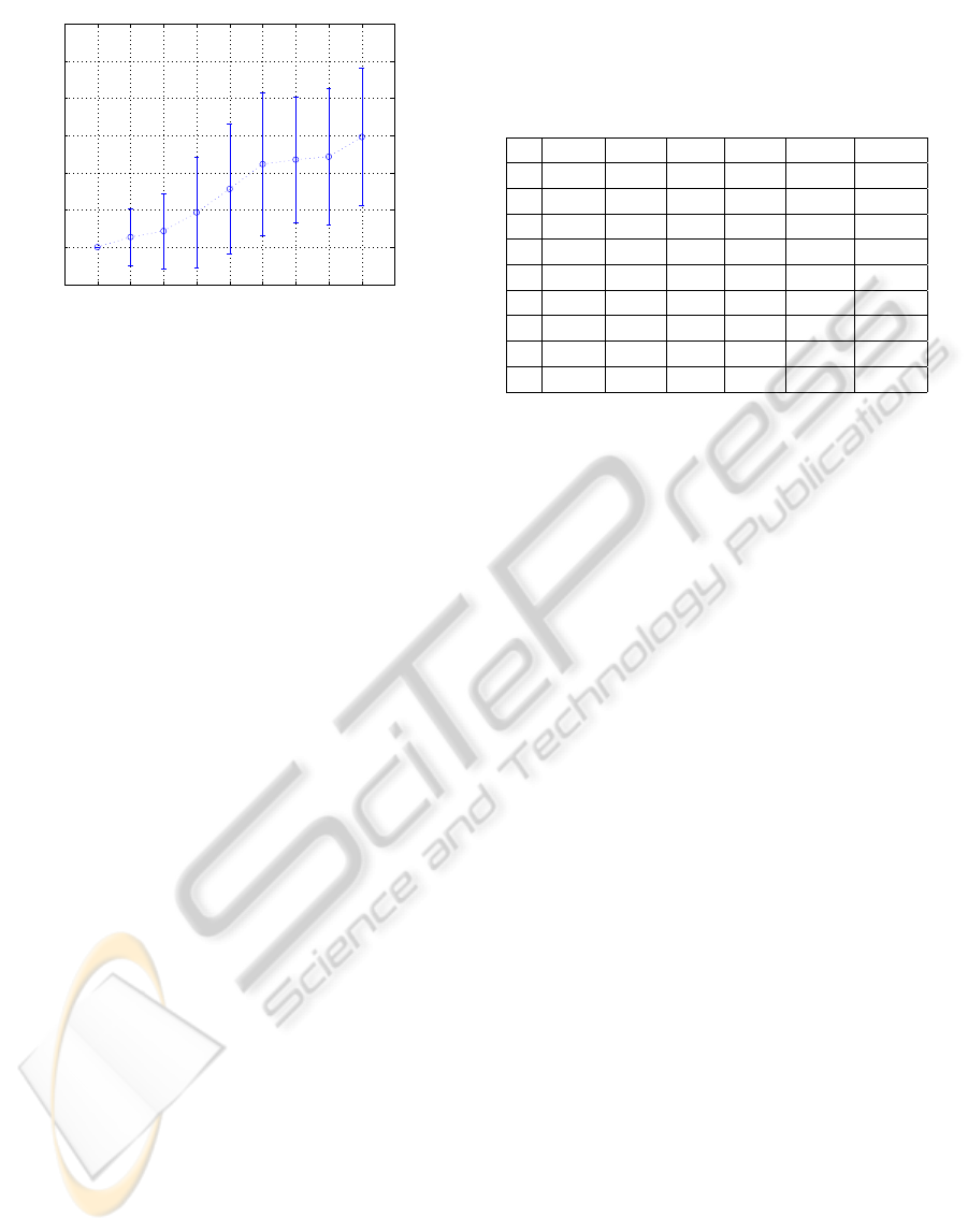
Figure 1: Maximum overlap between pairs of clusters ver-

sus number of clusters c for the Gaussian 2D problems. For

a given c the average over 100 problems and its standard

deviation are shown.

single cluster, represented by the mixture component

that most likely explains it. For the 2D Gaussian prob-

lems we consider k ∈ {1, ...,13}. For the twonorm

problems we consider k ∈ {1,..., 4}. This means that

we end up with a set of 260 different clustering par-

titions (only 80 for the twonorm problems) that must

be validated in a subsequent stage. This validation is

performed using each of the 6 approaches described

in section 3. Each approach leads to a single selected

partition for each of the problems.

5.2 Evaluation of the Results

To measure the quality of a validated partition, and

extensively the quality of a given validation approach,

we compare the number of regions in the partition

with the real number of clusters in the problem. We

consider the number of problems for which a given

validation approach provides a partition into the cor-

rect number of regions. Additionally, in some cases

we also compute the average number of regions to

have an idea of whether the validation index tends to

under or over-estimate the number of clusters.

Finally, in order to measure the intrinsic difﬁculty

of a given clustering problem, we consider the max-

imum overlap between any two clusters in the prob-

lem. We measure the overlap between two clusters

as the Bayes error for a two-class classiﬁcation prob-

lem where each cluster is one class. For the Gaussian

2D problems, this overlap increases with the number

of clusters because the total amount of space is ﬁxed

(see ﬁgure 1). The twonorm problem, on the other

hand, is designed such that the Bayes error is con-

stant (≈ 0.023) and independent of the dimension, so

all the problems have in this case the same intrinsic

difﬁculty.

Table 1: Gaussian problems in 2D. Number of problems

correctly validated by each of the six validation approaches

considered. The ﬁrst column, c, represents the actual num-

ber of clusters. The number of problems for a given c is

100.

c AIC BIC D J

D J

1 48 99 72 88 100 100

2 5 91 11 24 84 95

3 1 91 10 21 75 91

4 1 83 3 20 66 84

5 2 79 9 20 46 61

6 3 83 10 17 37 45

7 3 72 13 13 24 35

8 5 66 12 17 29 32

9 3 42 16 18 16 16

6 RESULTS

6.1 Gaussian Clusters in 2D

In table 1 we show the number of problems for which

each validation technique provides the correct num-

ber of clusters. Each row shows the results for a given

number of real clusters in the problem. There are 100

different problems for each number of clusters, there-

fore the maximum possible value in the table is 100.

We see that the negentropy-based approaches D J

and D J

outperform the classical BIC index only for

problems with a small number of clusters (c ≤4). Of

these, the D J

provides slightly better results. The

BIC index is the best for high number of clusters. The

D J

, D J

and AIC indices perform very poorly for all

the problems.

In table 2 we show the average number of clus-

ters for the solutions selected by each of the methods.

Note that, in spite of ﬁnding a correct solution in more

occasions, BIC presents a stronger tendency to over-

estimate the number of clusters when it fails. In such

a situation, the indices D J

and D J

tend to under-

estimate the number of clusters. From a clustering

perspective, this kind of error is in more accordance

with intuition: it seems more plausible to merge two

highly overlapping clusters than to split a single clus-

ter into two components. It was shown in ﬁgure 1

that the maximum overlap increases with the number

of clusters. This could explain the observed loss of

performance of D J

and D J

with increasing c. Fi-

nally, the D J

, D J

and AIC indices tend to overesti-

mate the number of clusters even in the low overlap

regime.

In ﬁgure 2 we show how the overlap is distributed,

both for the correctly and the incorrectly validated

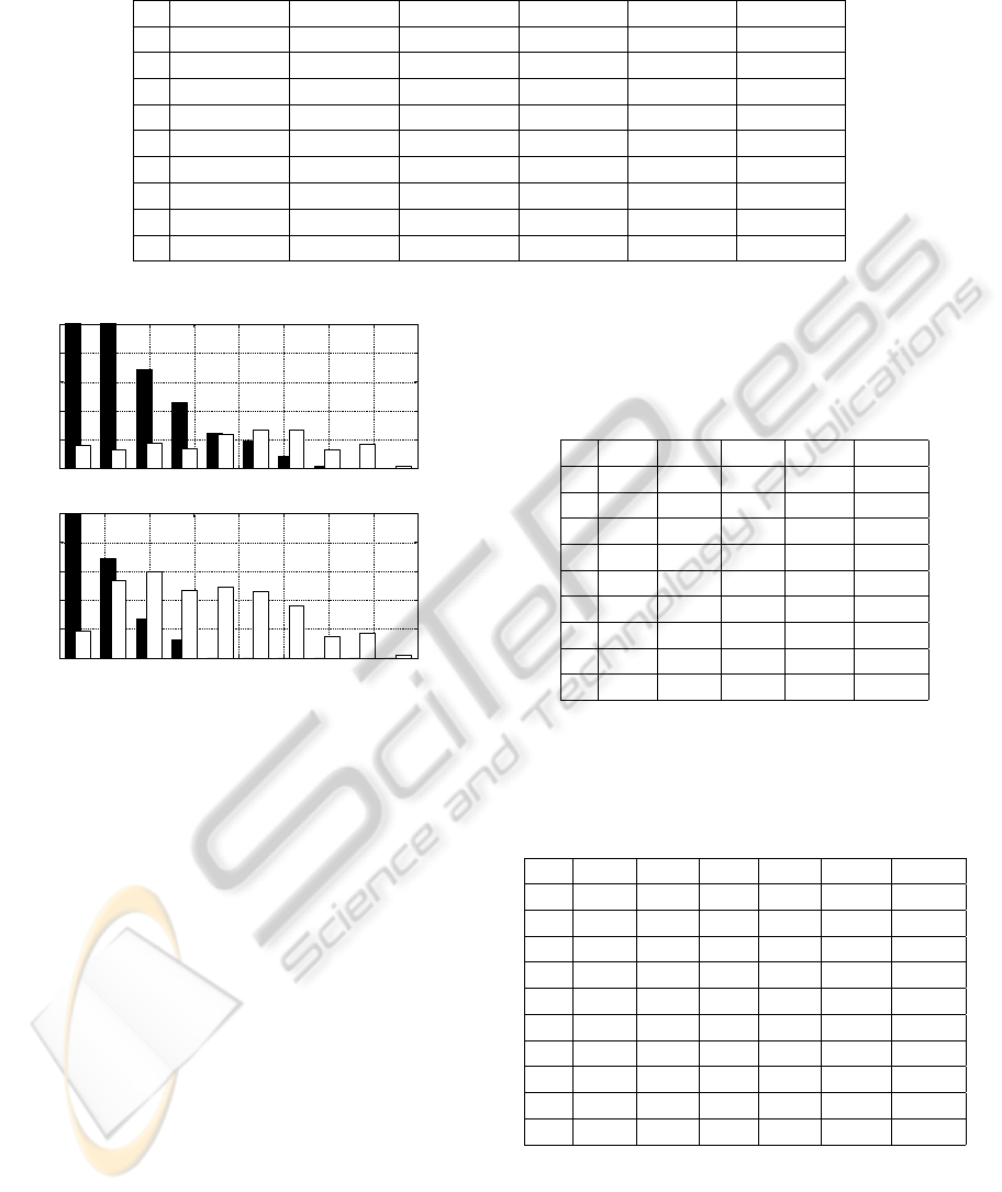
Table 2: Gaussian problems in 2D. Average number of clusters in the validated partitions for each of the six validation

approaches considered. The column labeled c shows the actual number of clusters.

c AIC BIC D J

D J

1 2.5 ± 1.7 1.0 ± 0.2 1.8 ± 1.4 1.4 ± 1.1 1.0 ± 0.0 1.0 ± 0.0

2 4.7 ± 1.2 2.1 ± 0.6 4.0 ± 1.7 3.3 ± 1.6 1.8 ± 0.4 1.9 ± 0.2

3 6.0 ± 1.0 3.1 ± 0.4 4.9 ± 1.6 4.3 ± 1.5 2.7 ± 0.5 2.9 ± 0.3

4 6.8 ± 1.1 4.0 ± 0.5 6.2 ± 1.8 5.3 ± 1.7 3.6 ± 0.7 3.8 ± 0.4

5 7.6 ± 1.1 4.9 ± 0.4 6.5 ± 2.0 5.8 ± 1.8 4.3 ± 0.9 4.5 ± 0.6

6 8.8 ± 1.2 5.8 ± 0.4 7.6 ± 2.0 7.2 ± 1.7 5.0 ± 0.9 5.3 ± 0.8

7 9.7 ± 1.1 6.8 ± 0.6 8.6 ± 2.1 7.8 ± 1.8 5.8 ± 1.0 6.1 ± 0.9

8 10.8 ± 1.2 7.8 ± 0.8 9.9 ± 2.0 9.1 ± 1.9 6.9 ± 1.3 6.7 ± 1.2

9 11.7 ± 1.2 8.8 ± 1.0 10.2 ± 2.2 9.6 ± 2.0 7.6 ± 1.5 7.4 ± 1.1

0 0.05 0.1 0.15 0.2 0.25 0.3 0.35 0.4

100

BIC

overlap

# occurrences

0 0.05 0.1 0.15 0.2 0.25 0.3 0.35 0.4

100

Negentropy

overlap

# occurrences

Figure 2: Distribution of overlaps for correctly (black ﬁlled)

and incorrectly (white ﬁlled) validated problems by each of

the two methods BIC (top) and D J

(bottom). The highest

bars have been truncated for the sake of clarity.

problems by each of the two methods BIC (top) and

D J

(bottom). The distributions for D J

are similar

to those for D J

(not shown). Observe that D J

able to assess the correct number of clusters only for

small overlap. The number of failures is also reduced

in this small overlap region. This is in clear contra-

diction with the observation for BIC, which is able to

ﬁnd the correct partition even in high overlap regimes.

If we recompute the values shown in table 1 tak-

ing into account only the problems whose maximum

overlap is below a given threshold t, we obtain the re-

sults shown in table 3. The value of the threshold has

been ﬁxed to t = 0.03. The column labeled NP shows

the number of problems that satisfy this restriction for

a given c. Note that now there is almost no difference

between the results provided by BIC and D J

Table 3: Gaussian problems in 2D. Number of problems

correctly validated by each of the six validation approaches

considered. Only problems with overlap lower than t = 0.03

are considered. The column labeled NP shows the number

of problems that satisfy this constraint for a given c.

c NP AIC BIC D J

D J

1 100 48 99 100 100

2 86 2 78 75 86

3 79 1 72 65 79

4 63 0 54 50 62

5 42 0 40 32 40

6 28 1 27 19 24

7 12 0 10 7 10

8 16 1 14 12 12

9 7 0 4 4 3

Table 4: Twonorm problems. Number of problems correctly

validated by each of the six validation approaches consid-

ered. The ﬁrst column, d, indicates the dimensionality of

the problem. The number of problems for a given d is 100.

d AIC BIC D J

D J

2 31 100 80 89 100 100

4 5 100 38 55 100 100

6 1 100 2 10 100 100

8 0 100 0 2 100 100

10 0 9 0 0 100 100

12 0 0 0 0 100 100

14 0 0 0 0 100 100

16 0 0 0 0 100 97

18 0 0 0 0 93 81

20 7 0 0 0 62 76

6.2 Twonorm Problems

The twonorm problems considered here present an

overlap of approximately 0.023. This falls below

the threshold t = 0.03 used previously to ﬁlter high

Table 5: Twonorm problems. Average number of clusters in the validated partitions for each of the six validation approaches

considered. The ﬁrst column shows the dimensionality of the problem.

d AIC BIC D J

D J

2 3.0±0.8 2.0±0.0 2.3±0.8 2.1 ±0.4 2.0±0.0 2.0 ±0.0

4 3.6±0.6 2.0 ±0.0 2.8±0.7 2.6±0.7 2.0±0.0 2.0±0.0

6 3.8±0.4 2.0 ±0.0 3.6±0.5 3.4±0.7 2.0±0.0 2.0±0.0

8 3.8±0.4 2.0 ±0.0 3.9±0.3 3.6±0.5 2.0±0.0 2.0±0.0

10 3.7±0.4 1.1±0.3 4.0 ±0.1 3.8±0.4 2.0±0.0 2.0±0.0

12 3.8±0.4 1.0±0.0 4.0 ±0.0 4.0±0.2 2.0±0.0 2.0±0.0

14 3.8±0.4 1.0±0.0 4.0 ±0.0 4.0±0.1 2.0±0.0 2.0±0.0

16 3.6±0.5 1.0±0.0 4.0 ±0.0 4.0±0.0 2.0±0.0 2.0±0.2

18 3.4±0.5 1.0±0.0 4.0 ±0.0 4.0±0.0 2.1±0.3 2.2±0.4

20 3.2±0.5 1.0±0.0 4.0 ±0.0 4.0±0.0 2.4±0.5 2.2±0.4

overlap problems, which means that the two clusters

are quite well separated. The difﬁculty in this case

arises from the high dimensionality. The results for

these problems are shown in tables 4 and 5. The

ﬁrst column in both tables is the dimension. Table 4

shows the number of problems for which each of the

validation methods provides a solution with 2 clus-

ters. Table 5 shows the average number of clusters in

the assessed solutions. All the validation approaches

show a loss of performance when the dimension of the

problems increases, but the D J

and D J

indices

are more robust than the others. BIC starts to fail at

d = 10, experimenting a sudden loss of accuracy. For

higher dimensions it tends to select one single cluster.

On the other hand, D J

and D J

are very accurate

even for d = 16, and their loss of accuracy for higher

dimensions is more gradual. Finally, the D J

, D J

and

AIC approaches provide very poor results, and show

a strong tendency to overestimate the number of clus-

ters.

7 CONCLUSIONS

The aim of this paper was to systematically study

the performance of negentropy-based cluster valida-

tion in synthetic problems with increasing dimension-

ality. Negentropy-based indices are quite simple to

compute, as they only need to estimate the probabil-

ities and the log-determinants of the covariance ma-

trices for each cluster. However, the computation of

the log-determinants in regions with small number of

points introduces a strong bias that must be corrected

in order to properly estimate the negentropy index. A

heuristic based on a formal analysis of the bias can be

obtained to alleviate this effect.

In this paper we reﬁned the correction of the ne-

gentropy index proposed in (Lago-Fern´andez et al.,

2011) in order to quantify the conﬁdence levels of

the index value, thus obtaining a new, more formal

heuristic for the validation of clustering partitions.

Then we studied the performance of this and other

negentropy-based validation approaches in problems

with increasing dimensionality, and compared the re-

sults with two well established techniques such as

BIC and AIC. The performance of BIC in problems

where the ratio of the number of points to the di-

mension is high, is quite good. For problems where

there are clusters with a high overlap, it clearly out-

performs the negentropy-based indices. This was ex-

pected since BIC is optimal for Gaussian clusters,

which is the case for the synthetic data considered

here. The AIC criterion seems to produce very bad

results for the set of problems considered, providing a

strong overestimation of the number of clusters in all

the cases. Negentropy-based indices are designed for

crisp clustering, and they seek to detect compact and

well separated clusters. When we consider only prob-

lems where the clusters are not highly overlapped, the

performances of BIC and the negentropy-based index

are quite similar.

In order to test the behavior of the indices as

a function of the dimensionality, we constructed

a clustering benchmark database based on the

twonorm classiﬁcation problem (Breiman, 1996).

This database is generated using two Gaussian clus-

ters of increasing dimensionality but constant degree

of overlap. The number of points in each cluster is

constant independently of the dimension. Therefore,

the effect of the dimensionality on the performance

of the indices is isolated. As the dimensionality in-

creases, the performance of BIC degrades quickly,

but the performance of the negentropy-based index

is quite stable, ﬁnding the correct solution for all the

problems up to d = 16, and experimenting a gradual

degradation for higher dimension.

In conclusion we showed, using the synthetic

database twonorm, that our approach to negentropy-

based validation can outperform AIC and BIC in

problems where the ratio of the number of points

to the dimension is not high, which is a very com-

mon situation in most real applications. New exper-

iments with other databases are required in order to

check if this property is general. We expect that this

ﬁnding will be more accentuated in benchmarks with

non Gaussian clusters (Biernacki et al., 2000; Lago-

Fern´andez et al., 2009). This will be the subject of

future work.

ACKNOWLEDGEMENTS

The authors thank the ﬁnancial support from DGUI-

CAM/UAM (Project CCG10-UAM/TIC-5864).

REFERENCES

Abramowitz, M. and Stegun, A. (1965). Handbook of math-

ematical functions. Dover, New York.

Akaike, H. (1974). A new look at the statistical model iden-

tiﬁcation. IEEE Trans. Automatic Control, 19:716–

723.

Biernacki, C., Celeux, G., and Govaert, G. (2000). Assess-

ing a mixture model for clustering with the integrated

completed likelihood. IEEE Trans. Pattern Analysis

Machine Intelligence, 22(7):719–725.

Breiman, L. (1996). Bias, variance, and arcing classiﬁers.

Technical Report 460, Statistics Department, Univer-

sity of California, Berkeley, CA, USA.

Fraley, C. and Raftery, A. (1998). How many clusters?

which clustering method? answers via model-based

cluster analysis. Technical Report 329, Department

of Statistics, University of Washington, Seattle, WA,

USA.

Gordon, A. (1998). Cluster validation. In Hayashi, C.,

Ohsumi, N., Yajima, K., Tanaka, Y., Bock, H., and

Baba, Y., editors, Data science, classiﬁcation and re-

lated methods, pages 22–39. Springer.

Lago-Fern´andez, L. F. and Corbacho, F. (2010). Normality-

based validation for crisp clustering. Pattern Recogni-

tion, 43(3):782–795.

Lago-Fern´andez, L. F., S´anchez-Montan´es, M. A., and Cor-

bacho, F. (2009). Fuzzy cluster validation using the

partition negentropy criterion. Lecture Notes in Com-

puter Science, 5769:235–244.

Lago-Fern´andez, L. F., S´anchez-Montan´es, M. A., and Cor-

bacho, F. (2011). The effect of low number of points

in clustering validation via the negentropy increment.

Neurocomputing, 74(16):2657–2664.

Misra, N., Singh, H., and Demchuk, E. (2005). Estimation

of the entropy of a multivariate normal distribution.

Journal of Multivariate Analysis, 92(2):324–342.

Schwartz, G. (1978). Estimating the dimension of a model.

Annals of Statistics, 6:461–464.

Xu, R. and II, D. W. (2005). Survey of clustering algo-

rithms. IEEE Trans. Neural Networks, 16(3):645–678.