
MULTI-HOP POSITIONING
Relative Positioning Method for GPS Wireless Sensor Network
Masayuki Saeki
1
and Kenji Oguni
2
1
Tokyo University of Science, Yamazaki 2641, Noda-shi, Chiba, Japan
2
Keio University, Yagami 3-14-1, Kohoku-ku, Yokohama-shi, Kanagawa, Japan
Keywords: GPS, Relative positioning, Wireless sensor network, Displacement monitoring.
Abstract: This paper presents a relative positioning method, called “multi-hop positioning”, which is suitable for raw
GPS data collected by densely deployed L1 GPS receivers. The wireless sensor network employing an
affordable L1 GPS receiver has been developed by the authors for monitoring displacement of large civil
structures with high spatial resolution. In general, relative positioning of GPS sensors are performed
between a single reference point and sensor nodes. On the other hand, in the newly developed approach,
relative positioning is performed between all pair of sensor nodes in the network. Then, the best set of
relative position vectors is selected to determine the location of sensor nodes. Experiments have been
conducted using 53 sensor nodes equipped with an affordable L1 GPS receiver and the collected data are
analysed by using the proposed method in a post-processing manner. The results show that the success rate
of relative position estimate is considerably improved compared with the conventional approach.
1 INTRODUCTION
Displacement monitoring of large infrastructures
such as artificial island, embankment and reclaimed
land is very important. This work is operated for
controlling quality and ensuring safety. In general,
displacement monitoring is performed by survey
work or an automated monitoring system in which
accurate instruments are networked with cables and
the displacements are monitored remotely. Although
the automated monitoring system could replace the
survey work for reducing the monitoring cost, the
application examples are still limited. One of the
disadvantages of the current automated system is its
high cost. Very expensive instruments such as a
laser displacement meter or a high performance GPS
(Global Positioning System) receiver is employed to
detect the displacement in sub-centimetres accuracy.
For the dense displacement monitoring of large
civil infrastructures, a cost-effective system should
be developed. The combination of wireless sensor
network and an affordable L1 GPS receiver can be a
possible solution to this problem. Besides, the
wireless sensor network has big advantages not only
in cost but also in robustness and workability (Lynch,
2004). Therefore, we have been developing the
system of wireless sensor network using an
affordable L1 GPS receiver (Saeki, 2008). We call
this system GWSN (GPS Wireless Sensor Network).
This system consists of a central server and many
sensor nodes equipped with an affordable L1 GPS
receiver. Each sensor node collects raw GPS data
according to the command from the central server
and sends their data back to the server. The relative
positions of the sensor nodes from a reference point
are analyzed in the server. The displacements of the
sensor nodes are estimated as the change of position
from the initial state.
Since the sensor node runs using a small battery
and/or additional harvested energy, the total energy
consumption should be suppressed. Considering the
high energy consumption of the GPS receiver, the
observation time should be minimized. On the other
hand, to improve the accuracy of positioning, the
observation should be performed as long as possible.
Clearly this system has the trade-off relationship
between the accuracy and the energy consumption.
Therefore we have tried to develop a new relative
positioning method which gives accurate relative
position with short data length.
This paper presents a relative positioning method
suitable for the data collected by the densely
deployed GPS receivers with short data length. In
this method, the location of the sensor node is
361
Saeki M. and Oguni K..
MULTI-HOP POSITIONING - Relative Positioning Method for GPS Wireless Sensor Network.
DOI: 10.5220/0003798503610368
In Proceedings of the 2nd International Conference on Pervasive Embedded Computing and Communication Systems (PECCS-2012), pages 361-368
ISBN: 978-989-8565-00-6
Copyright
c
2012 SCITEPRESS (Science and Technology Publications, Lda.)

estimated as a sum of the relative position vectors.
Relative positioning is performed between all pair of
sensor nodes in the network and the optimal sum of
relative position vectors is selected to determine the
location of sensor nodes. To assess the performance
of our method, experiments have been conducted
using 53 wireless sensor nodes. The collected data
are analysed by using the proposed method in a post-
processing manner. The results show that the
success rate of estimating the relative positions is
considerably improved compared with the
conventional approach.
2 RELATED WORK
GPS-less localization method for large networks of
wireless sensor nodes has been intensively studied
by many researchers. For example, Bulusu et al.,
(2000) evaluates the effectiveness of a simple
connectivity metric method for localization in
outdoor environments. Moor et al., (2004) presents a
linear-time algorithm for localizing sensor network
nodes in the presence of range measurement noise
and demonstrates the algorithm on a physical
network. These results show that the accuracy
depends on the scale of distribution and is not high
enough for monitoring displacements of large civil
infrastructures, which needs a few centimetres to
sub-centimetres accuracy.
Many displacement monitoring systems using L1
GPS receivers are developed and demonstrated in a
real field. Gassner et al., (2002) developed a GPS-
based continuous monitoring system and applied it
to landslide monitoring. Shimizu, (2003) developed
a monitoring system and applied it to large open
quarries and landslide slopes. Seynat, et al., (2004)
developed the monitoring system, which uses a low
cost GPS receiver and a radio link, and applied their
system to volcano monitoring. These demonstrations
show that displacement monitoring using L1 GPS
receivers might be possible in terms of accuracy.
In order to deploy the sensor nodes densely
covering a large infrastructure, the cost for a single
observation point should be decreased further. So,
we have been developing the new displacement
monitoring system which combines the wireless
sensor network with an affordable L1 GPS receivers
connected to a small patch antenna which is
generally used for a mobile navigation (Saeki, 2008).
This combination enables us to decrease the cost of a
single observation point but brings about other
problems to be solved.
One of the problems is the energy consumption
of the GPS receiver. The sensor node of GWSN
keeps the GPS receiver off as long as possible to
save its battery. However, shortening observation
time results in the accuracy deterioration. To
overcome this problem, we have tried to develop a
new positioning method considering the condition of
dense sensor deployment.
The problem to determine the locations of many
GPS receiver simultaneously is known as network
adjustment (Han, 1995). In the network adjustment,
variance-covariance matrix between GPS sensors is
taken into account. However, it is so difficult to
estimate an appropriate variance-covariance matrix
in the application of a large infrastructure that
network adjustment might not be applicable.
3 GPS WIRELESS SENSOR
NETWORK
This section describes the outline of the present
system and the conventional relative positioning
method, and specifies the required technology.
3.1 Outline of the System
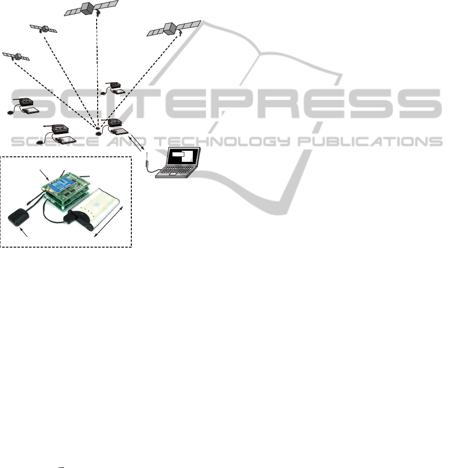
Figure 1 illustrates the schematic view of GWSN.
This system consists of a single central server and
many sensor nodes. The sensor node has a micro-
controller, a small wireless communication device, a
small battery and an affordable L1 GPS receiver.
The sensor nodes run according to the command
from the central server. After getting the command
to start observation, it turns on the GPS receiver
which outputs the raw binary messages to the micro-
controller every one second. The micro-controller
extracts the required data from the original binary
message and save them to the non-volatile memory.
The size of the original binary message is 266 bytes
and is compressed to 28 bytes in the present system.
After the sensor nodes collecting the data for several
minutes (e.g. 4 minutes), the central server orders
them to send their data back to itself. The locations
of the sensor nodes are analysed by the central
server in a post-processing manner.
In the prototype, a middle range series micro-
controller PIC16F877A (Microchip Technology
Inc.) is employed since any complex calculation is
not required. As an affordable L1 GPS receiver,
GT8032 (Furuno Electric co., ltd.) is used which is
capable of outputting L1 carrier phases in a Furuno
binary format. A small patch antenna is connected to
the receiver for saving cost. This kind of antenna is
PECCS 2012 - International Conference on Pervasive and Embedded Computing and Communication Systems
362
commonly used in an automotive navigation system
and never used for accurate positioning because the
measured carrier phases are very contaminated by
the antenna noises. The wireless communication
device of the prototype is MU1-1252 (Circuit
Design, Inc.) which uses the frequency band of 1252
MHz. The maximum distance of wireless
communication is 600 m with a line of sight at the
RF output power of 10 mW.
Figure 1: Schematic view of GPS wireless sensor network.
3.2 Conventional Relative Positioning
Method
In the present system, the relative position vector is
estimated by the static interferometry positioning
method which is widely used in a practical GPS
surveying to achieve centimetre-level accuracy.
3.2.1 Observation Equation
The relative position vector is estimated by
analysing the L1 carrier phases. In case of short
baseline, the DD (Double-Differenced) carrier
phases at time t,
(
)
, is modelled as follows
(Hofmann, 2001),
(
)
=
1
(, ) +
+
()
(1)
where ∗
represents the DD values for the GPS
satellites k, l and the sensor nodes i, j. is the
wavelength of L1 carrier waves,
(, ) is the DD
ranges between satellites and the nodes, is the
relative position vector of a sensor node,
is the
DD integer ambiguity and
is the noise. Eqn. (1)
is linearized by substituting =
+Δ and
applying the Taylor Expansion with respect to
.
Gathering Eqn. (1) corresponding to the different
sets of satellites forms the following simultaneous
equations.
(
)
= ()Δ + + ()
(2)
where
(
)
is the vector of the corrected DD carrier
phases, () is the design matrix. The unknowns in
Eqn. (2) are the correction terms for the position
vectors Δ and the vector of DD integer
ambiguities. Solving Eqn. (2) through the least mean
square method gives a float solution in which the
DD integer ambiguities are estimated as float values.
3.2.2 Integer Ambiguity Resolution
In order to achieve centimetre-level accuracy, the
DD integer ambiguities should be resolved as the
integer values. This solution is called fixed solution.
Denoting the float solution and the fixed solution as
and
, respectively, the fixed solution
is
estimated as the integer-valued vector which
minimizes the following objective function .
=
−
−
(3)
where
is the variance-covariance matrix of the
float solution
.
In general, the fixed solution is validated by
checking the ratio
/
where
and
are the
minimum residual and the second small one,
respectively. It is known that the larger ratio gives
the higher probability of selecting the correct DD
integer ambiguities. In the case that the ratio
/
is
greater than 3, the fixed solution is empirically
considered a correct solution. On the other hand, the
solution might be wrong with the smaller ratio, and
the wrong DD integer ambiguities might give more
than several centimetres to meters error to the
estimated position. In the general usage of GPS, the
data is logged until the ratio exceeds 3 to guarantee
the quality of solution. However, in the present
system, the observation time is limited to save
battery energy.
3.3 Required Component Technology
As mentioned above, it is preferable to measure the
GPS data longer for estimating the correct relative
GPS satellites
Central server
1
0
c
m
battery
small patch antenna
Sensor node
wireless communication module
MULTI-HOP POSITIONING - Relative Positioning Method for GPS Wireless Sensor Network
363

position vectors while the longer measurements
results in the higher energy consumption. Since the
sensor node should run for at least several months
without changing battery, it is needed to develop a
method to estimate the correct relative position
vectors with short data length.
As considering the affordable cost of this system,
the sensor nodes are expected to be densely
distributed over a large infrastructure. This dense
deployment might be a great advantage of the
present system. Therefore, we have tried to develop
a new relative positioning method considering the
dense deployment of the sensor nodes. In the
conventional approach, the relative position vectors
are individually estimated for each sensor node. And
the advantage of the dense GPS deployment is not
taken into account.
4 MULTI-HOP POSITIONING
Float solution is estimated by solving Eqn. (2) with
the assumption that the noise is white. The
assumption could be true in some pairs of sensor
nodes but could be false in other pairs. If the
surrounding conditions of the sensor nodes are very
similar to each other, the noises also become very
similar. In the case, the noises can be cancelled out
in the double difference calculation and the residual
behaves as the white noise. On the other hand, when
the surrounding conditions of the sensors are
different from each other, the residuals of the noises
are not likely to be white. In this case, the accuracy
of the float solution becomes worse and the DD
integer ambiguities are not correctly resolved in the
minimization problem of Eqn. (3). This leads to the
wrong relative position vectors. Therefore, it is very
important to select a good pair of sensor nodes
whose noises are very similar to each other.
4.1 Basic Idea of the Proposed Method
Suppose that three sensor nodes are there and the
noises are different from each other but the noise of
node 3 has some similarities to those of node 1 and 2.
This situation often happens in actual observations
when many sensor nodes are deployed densely. In
such case, the relative position of node 2 from 1 is
likely to be estimated wrong and the ratio
/
becomes small since the noises are not cancelled out
in the DD calculation. On the other hand, the relative
position of node 3 could be estimated correctly and
the ratio becomes larger than that of node 2. This
situation is schematically drawn in Figure 2(a). Two
relative position vectors and ratios are described on
the figure. In this example, node 2 is unsuccessfully
estimated.
Figure 2: Simple example of the relative position vectors
estimated by the conventional method (a) on the left side
and the proposed method (b) on the right side.
In the above situation, the relative position of
node 2 is estimated wrong from node 1. However, it
can be estimated correctly by summing up the
relative position vectors as described in Figure 2(b).
Since the noise of node 2 has some similarities to
that of node 3, some parts of noises can be cancelled
out. Then it must yield better float solution and it
gives higher probability of selecting the correct
integer ambiguities. Then, the relative position of
node 2 from node 3 can be estimated in accurate.
In a real situation, there are many candidates of
the paths because many sensor nodes are distributed.
And besides, the ratios
/
might have similar
values. So there is a problem how to select the
optimal path with a convincing reason. To solve this
problem, we introduce the success probability into
the present approach. By comparing the success
probabilities evaluated for each path, the optimal
path can be selected convincingly.
4.2 Assumption of Success Probability
We assume that the success probability of resolving
the DD integer ambiguities is represented as a
function of ratio
/
. And the success probability
of a path can be estimated as the products of the
success probabilities of the corresponding relative
position vectors. In this subsection, we empirically
estimate the function relating the success probability
and the ratio
/
.
4.2.1 Experiment and Data Analysis
Figure 3 shows a look of the experiment conducted
on the concrete roof of a building March 3, 2008.
Since there are no obstacles over the site, it is
considered as an ideal condition. In the experiment,
Node 1
2.0
1.1
N
ode 2
Node 3
Node 1
2.0
1.5
Node 2
Node 3
(a) (b)
PECCS 2012 - International Conference on Pervasive and Embedded Computing and Communication Systems
364
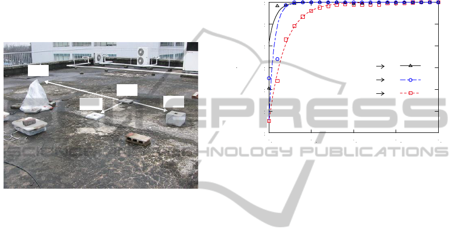
four sensor nodes are deployed in the different
manner. Two GPS antennas are fixed on the flat
plane of thin concrete block (ID1 and ID2) and the
other antenna is mounted on the concrete block with
different height (ID3). Another antenna is fixed at
the tripod (ID4). These various antenna conditions
are set for causing different antenna noises. For
example, the antenna noises of ID1 and ID2 are so
similar that the noises are effectively cancelled out
in the DD calculation. On the other hand, the
antenna noises of ID1 and ID4 are apparently
different and cannot be eliminated in the analysis.
Figure 3: Photo of the experiment conducted for collecting
raw GPS data with the different antenna conditions.
The raw GPS data are sampled for 24 hours at
1Hz sampling rate and are saved on a laptop. The
data is analysed in a post-processing manner. In the
analysis, relative position vectors of ID1-2, ID1-3
and ID1-4 are estimated.
In the analysis, the data with the length of 240
seconds is picked up from the continuous data and
analysed by means of the conventional relative
positioning. If the estimated location of sensor node
is within 3 centimetres from the most possible
position, this estimation is counted as a success. The
same operation is applied to the next data shifted
from the previous data by 1 second. These processes
are carried out 86400 times for each sensor node.
The estimated results are classified depending on the
value of the ratio
/
. The success probability,
which is defined as the ratio of the frequency of
successes to trials in this paper, is estimated for each
class.
4.2.2 Success Probability of a Single Vector
The success probabilities obtained from the above
analysis are plotted in Figure 4. The marks of
triangle, circle and square represent the results of
ID1-2, ID1-3 and ID1-4, respectively. Three curves
are the corresponding success probability functions
which are estimated by the least square method. In
this paper, the success probability function
(
)
is
assumed to be the following function.
(
)
=1.0−
(4)
where is the ratio
/
, and are the unknown
parameters to be estimated.
Figure 4: The relationship between the success probability
and the ratio
/
.
As shown in Figure 4, the success probability of
ID1-4 has smaller values compared to that of ID1-2
especially at the small ratio
/
. This means that
the success probabilities depend on the conditions of
antenna noises as well as the ratio. In the following
simulations, the curve corresponding to the case of
ID1-4 is used because it mostly represents a realistic
condition among them.
4.2.3 Success Probability of a Path
In the proposed method, a relative position vector of
sensor node is obtained by connecting other relative
position vectors. The success probability of the path
can be evaluated by multiplying the success
probabilities of the corresponding relative position
vectors.
(
)
=(
)(
)⋯(
)
(5)
where
is the ratio
/
of relative position vectors
constituting the path.
4.3 Optimal Path Finding by Dijkstra’s
Algorithm
The optimal path should be reasonably selected from
the numerous candidates by searching the path with
the maximum success probability. In the proposed
ID4
ID2
ID1
ID3
40
50
60
70
80
90
100
1.0 1.5 2.0 2.5 3.0
ratio, J/J
2
1
Success P
r
obabili
t
ies [%]
14
12
13
MULTI-HOP POSITIONING - Relative Positioning Method for GPS Wireless Sensor Network
365
method, Dijkstra’s algorithm is used as a search
algorithm (Wiitala, 1987). This algorithm is widely
used in many applications such as network routing
protocols or mobile navigation systems to find the
shortest (or lowest cost) path efficiently.
Dijkstra’s algorithm is applicable to the present
problem with a small modification. In the proposed
method, the optimal path is searched not for the
shortest length but for the maximum success
probabilities.
5 DEMONSTRATIONS
In order to investigate the performance of the
proposed method, we conduct two experiments and
analyse the data using both the conventional and the
proposed method. This section describes the details
of experiments and the results.
5.1 Experiment Described in Section 4
The data, collected in the experiment described in
the previous section, are analysed. In this analysis,
the sensor node ID1 is set to be a reference point and
the relative positions of the other sensor nodes are
estimated by using the conventional and the
proposed method. The data length is set 240 seconds
and the estimation is carried out 86400 times in the
same manner as mentioned in the section 4.2.1. If
the estimated position is within 3 centimetres from
the most possible position, the estimation is counted
as a success. And the success rate is estimated by
dividing the frequency of successes by trials. Table 1
shows the comparison of the success rates. The
success rate of ID2 slightly decreases but the other
success rates of ID3 and ID4 are improved. Overall,
it is said that the success rates are improved by using
the proposed method.
Table 1: Comparison of the success rates estimated by
analysing the data collected in the experiment described in
section 4.
Conventional Proposed
ID1 to 2 100.00 99.94
ID1 to 3 99.91 100.00
ID1 to 4 94.99 95.70
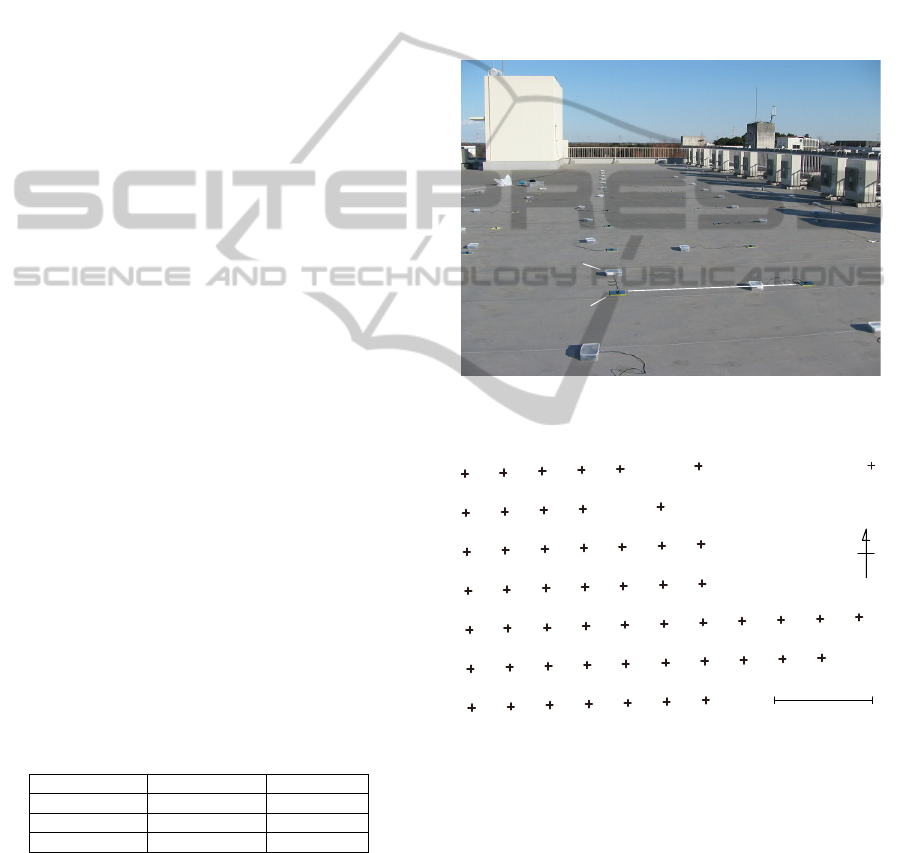
5.2 Experiment using 53 Sensor Nodes
5.2.1 Experimental Condition
Next, we conduct an experiment using 53 sensor
nodes to make sure that the proposed method works
well in case of dense deployment. In this experiment,
53 sensor nodes are arranged every two meters in a
grid on the rooftop of a building as shown in Figure
5 and 6. Some of GPS antennas are intentionally
located in the vicinity of the obstacles (the outdoor
equipment of air-conditioner shown in the right in
Figure 5 and the white building behind the sensor
nodes). This deployment of the antenna is for non-
uniform signal environment and corresponding
variety of the antenna noises. The raw GPS data are
collected for 4 minutes and gathered to the central
server via wireless communication.
Figure 5: Photo of the experiment conducted for collecting
GPS data using densely deployed GPS receivers.
Figure 6: Arrangement of 53 sensor nodes in a grid.
5.2.2 Results of Analysis
In the analysis, the conventional and the proposed
approach are performed setting every sensor node as
a reference point because the results of analysis
depend on the choice of the reference point. So, the
position of each sensor node is estimated 52 times in
this analysis. Table 2 shows the worst five success
rates which are estimated using the conventional
approach and the success rates of corresponding
sensor nodes improved by the proposed method. All
Sensor node
GPS antenna
2
m
From West to East
5m
1
2
3
4
5
6
7
8
9
10
11
12
13
14
15
16
17
18
19
20
21
22
23
24
25
26
27
28
29
30
31
32
33
34
35
36
37
38
39
40
41
42
43
44
45
46
47
48
49
50
51
52
53
N
GPS Antenna
PECCS 2012 - International Conference on Pervasive and Embedded Computing and Communication Systems
366

sensor nodes listed up on the Table 2 locates near
the obstacles which cause different antenna noises.
The different antenna noises decrease the success
rates. However, the success rates obtained using the
proposed method are all improved to 100.00% in
this analysis. The multi-hop positioning method
works well especially in case of dense deployment
of sensor nodes because it is easier to find out the
best pairs of sensor nodes which include almost the
same antenna noises.
Table 2: Comparison of success rates in case of the
experiment using 53 sensor nodes.
Conventional Proposed
ID29 43.40 100.00
ID13 69.81 100.00
ID36 86.79 100.00
ID17 88.68 100.00
ID09 90.57 100.00
One of the worst cases in case of applying
conventional method is obtained if the sensor node
of ID17 is set a reference point. The estimated
locations are shown in Figure 7. The success
probabilities calculated by Eqn. (4) are also plotted
in the figure. In this estimation, 6 relative position
vectors are mistakenly determined and the success
probabilities are relatively small in the vicinity of
obstacles. Since the antenna of the sensor node of
ID17 is fixed among the white building and the
outdoor equipment of air-conditioners, the antenna
noises are considered to be very different from the
others.
Figure 7: Locations of the sensor nodes estimated by the
conventional method with the reference point ID17.
The results obtained by the proposed method
with the reference point of ID17 are shown in Figure
8. We can easily see that the proposed method
outputs better solution. All relative positions are
correctly determined and the success probabilities
are improved greater than 0.99 even though the
reference point seems to be set under the noisy
condition. Figure 9 describes the optimal path
determined by the search algorithm. The number of
connections of the relative position vectors is at
most 11 in this case.
Figure 8: Locations of the sensor nodes estimated by the
proposed method with the reference point being in the
worst condition (ID17).
Figure 9: The optimal path found out by the search
algorithm in case of setting ID17 the reference point.
6 CONCLUSIONS
This paper presents the relative positioning method,
called multi-hop positioning, which is suitable for
the data collected by the densely deployed GPS
sensors. We introduce the success probabilities into
the estimation of relative position vectors. The
relative position of sensor nodes from a reference
point is calculated as a sum of relative position
vectors. The optimal path, which connects the
relative position vectors, is selected by the Dijkstra’s
algorithm with maximizing the success probability.
We demonstrate the proposed method analysing the
experimental data. One experiment is carried out for
24 hours using 4 sensor nodes and the other
experiment using 53 sensor nodes. The analytical
results show that the success rates of estimating the
correct relative position using the proposed method
0.997
0.988
0.870
0.999
0.524
1.000
0.998
0.992
0.956
0.990
0.999
1.000
0.665
0.493
0.998
0.970
0.000
1.000
1.000
0.960
0.904
0.999
1.000
1.000
1.000
0.938
0.987
1.000
0.690
1.000
1.000
1.000
0.987
1.000
0.997
0.482
0.971
0.999
0.835
0.999
0.998
1.000
1.000
1.000
0.961
0.999
0.997
0.992
0.998
1.000
1.000
1.000
0.981
GPS Antenna
Estimated position
1.000
1.000
1.000
1.000
1.000
1.000
1.000
1.000
0.993
1.000
1.000
1.000
1.000
1.000
1.000
1.000
1.000
1.000
1.000
0.997
1.000
1.000
1.000
1.000
1.000
1.000
1.000
1.000
1.000
1.000
1.000
1.000
1.000
1.000
1.000
1.000
1.000
1.000
1.000
1.000
1.000
1.000
1.000
1.000
1.000
1.000
1.000
1.000
1.000
1.000
1.000
1.000
1.000
MULTI-HOP POSITIONING - Relative Positioning Method for GPS Wireless Sensor Network
367

is considerably improved compared with the
conventional approach.
REFERENCES
Bulusu, N., Heidemann, J. and Estrin, D., 2000, GPS-less
low-cost outdoor localization for very small devices,
IEEE Personal Communications Magazine 7, 5, 28-34.
Gassner, G., Wieser, A. and Bruvver, F., 2002, GPS
software development for monitoring of landslides,
Proc. FIG XXII Congress, in CD-ROM.
Han, S. and Rizos, C., 1995, Selection and Scaling of
Simultaneous Baseline for GPS Network Adjustment,
or Correct Procedures for Processing Trivial Baselines,
Geomatics Research Australasia, No. 63, Dec., 51-66.
Hofmann, B. – Wellenhof, H. Lichtengger & Collins, J.,
2001. Theory and Practice, SpringerWienNewYork,
2
nd
edition.
Lynch, J.P., 2004, Overview of wireless sensors for real-
time health monitoring of civil structures, Proc. of the
4
th
International Workshop on Structural Control and
Monitoring, New York City, NY, USA.
Moore, D., Leonard, J., Rus, D. and Teller, S., 2004,
Robust Distributed Network Localisation with Noisy
Range Measurements, Proc. Second ACM SenSys.
Sadler, C. M. and Martonosi, M., 2006, Data Compression
Algorithms for Energy-Constrained Devices in Delay
Tolerant Networks, Proc. of the ACM Conference on
Embedded Networked Sensor Systems, Nov. 1-3.
Saeki, M., Oguni, K. and Hori, M., 2008, Development of
affordable GPS displacement monitoring system,
Proceeding of International Association for Bridge
Maintenance and Safety, 1906-1913.
Seynat, C., Hooper, G., Roverts, C. and Rizos, C., 2004,
Low-cost deformation measurement system for
volcano monitoring, Proceedings of The 2004
International Symposium on GNSS/GPS.
Shimizu, N., 2003, Continuous Displacement Monitoring
using Global Positioning System for Assessment of
Slope Stability, the 2
nd
Southeast Asian Workshop on
Rock Engineering, Hanoi, 136-145.
Wiitala, S. A., 1987, Discrete Mathematics, A Unified
Approach, McGRAW-HILL International editions,
Computer Science Series.
PECCS 2012 - International Conference on Pervasive and Embedded Computing and Communication Systems
368
