ANALYZING INVARIANCE OF FREQUENCY DOMAIN BASED
FEATURES FROM VIDEOS WITH REPEATING MOTION
Kahraman Ayyildiz and Stefan Conrad
Department of Databases and Information Systems
Heinrich Heine University Duesseldorf, Universit¨atsstraße 1, 40225 Duesseldorf, Germany
Keywords:
Motion Detection, Motion Recognition, Action Recognition, Repeating Movement, Video Classification,
Frequency Feature, Invariance, View-invariant.
Abstract:
This paper discusses an approach, which allows classifying videos by frequency spectra. Many videos contain
activities with repeating movements. Sports videos, home improvement videos, or videos showing mechanical
motion are some example areas. Motion of these areas usually repeats with a certain main frequency and sev-
eral side frequencies. Transforming repeating motion to its frequency domain via FFT reveals these frequency
features. In this paper we explain how to compute frequency features for video clips and how to use them for
classifying. The experimental stage of this work focuses on the invariance of these features with respect to
rotation, reflection, scaling, translation and time shift.
1 INTRODUCTION
Computer vision is a highly investigated research area
in computer science. Some aspects of this area are
video retrieval, video surveillance, human-computer
interfaces, object tracking and action recognition. All
of these topics play an important role for industry and
technique. Video databases for instance can be found
in major corporations or online video portals. More-
over video surveillance is needed to protect company
buildings, public places and private properties. Today
most digital video cameras use face tracking methods
in order to focus on faces and zoom into important
picture parts. So computer vision has relevance for
public and private life.
In this work we explain an approach, which is
able to detect, track and classify motion in video se-
quences. It is based on our previous research work
(Ayyildiz and Conrad, 2011) and improves its feature
extraction methods. Instead of considering single fre-
quency maxima now we utilize complete frequency
spectra derived from motion. Thus accuracies can
be improved and the system is more robust against
different types of invariance. Our approach focuses
on repeating motion and resulting frequency features.
It works for every motion type and is not limited to
human gait recognition as described in (Meng et al.,
2006; Zhang et al., 2004). The experimental part
of our research work analyzes invariance aspects of
these frequency features in order to find out, how ro-
bust the method works with varying camera settings.
This aspect is important, since video databases or-
dinarily contain videos with different camera angles,
zooming factors or object positions.
As a first step our method detects regions with mo-
tion for each frame. This regions lead to image mo-
ments for each frame, where a series of image mo-
ments represents a function. By a fast Fourier trans-
form (FFT) this function is transformed to its fre-
quency domain. A partitioning of this frequency do-
main into intervals gives different average amplitudes
for each interval. These average amplitudes are con-
sidered as features for each clip. Once feature vectors
are determined, a classifier can assign each clip to a
class.
In the following section we focus on the whole
process of video classification. We explain feature ex-
traction phase and classification phase stepwise. Fur-
thermorewe define image moments and so-called 1D-
functions for transformation in section 3. The basic
feature vectors AAFIs (Average Amplitudes of Fre-
quency Intervals) are explained in section 4. After-
wards we introduce our radius based classifier RBC in
section 5. The evaluation of our approach takes place
in section 6. The following section discusses work re-
lated to our approach, where the last section reviews
the presented methods.
659
Ayyildiz K. and Conrad S..
ANALYZING INVARIANCE OF FREQUENCY DOMAIN BASED FEATURES FROM VIDEOS WITH REPEATING MOTION.
DOI: 10.5220/0003798806590666
In Proceedings of the International Conference on Computer Vision Theory and Applications (VISAPP-2012), pages 659-666
ISBN: 978-989-8565-03-7
Copyright
c
 2012 SCITEPRESS (Science and Technology Publications, Lda.)

2 CLASSIFYING VIDEOS BY
AAFIS
In this section we explain methods used for our ap-
proach, where fig. 1 offers an overview of the differ-
ent stages.
videos
moments
1D-functions
transformation
AAFIs
features
regions of
movement
classifier
class
features
class A
class B
class C
DB
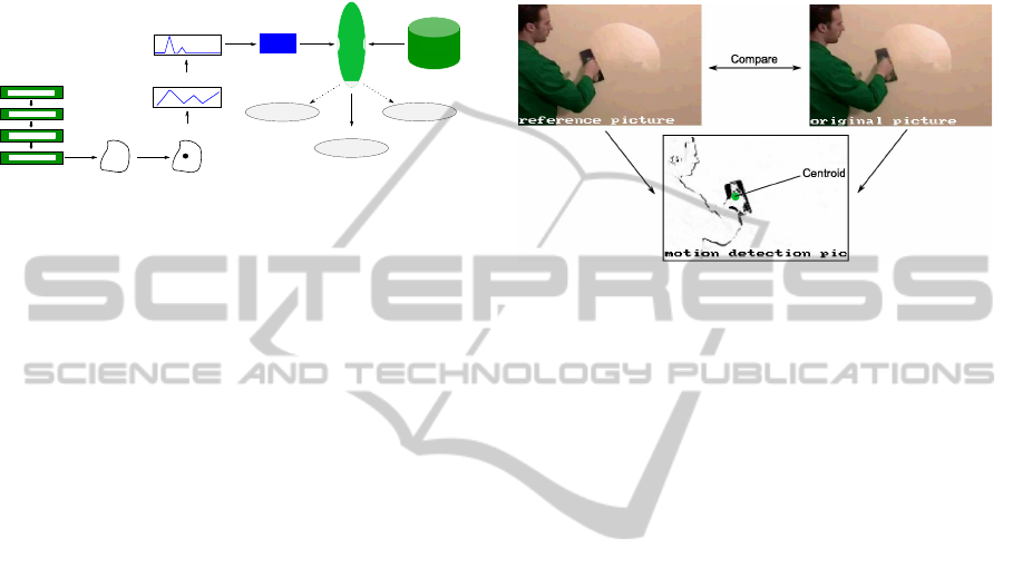
Figure 1: Flow diagram of whole classification process.
The goal of the whole classification process is to
classify video sequences with repeating movements
properly. Some examples for activity with repeating
movement are jumping, playing tennis or hammering.
First regions of movement are detected in every clip
for each frame. Regions are detected by measuring
the color differencesof pixels in two frames following
each other (see section 3.1). Based on these regions
we calculate image moments, where two types of mo-
ments are applied: centroids and pixel variances. A
chronological series of these moments are considered
as 1D-functions and represent the motion in a video
sequence. The FFT of one 1D-function reveals its
frequency domain. By partitioning the frequency axis
into intervals of same length, average amplitudes for
each interval are computed. We name these averages
AAFIs (Average Amplitudes of Frequency Intervals).
AAFIs constitute the final feature vectors for each clip
with respect to its motion. After determining the fea-
ture vector of a video its next class is computed by a
classifier.
3 IMAGE MOMENTS AND
1D-FUNCTIONS
Frequency spectra result from repeating motion in
video scenes and this motion has to be detected frame
by frame at first. Once the motion is localized image
moments and resulting 1D-functions can be figured.
Next we define regions of motion and explain how
these regions lead to 1D-functions.
3.1 Regions of Motion
Fig. 2 shows a person troweling a wall in two consec-
utive frames. By analyzing these two frames we de-
tect regions with motion. Color differences between
the first and the second frame are measured for each
pixel. If the color difference of a pixel exceeds a
predefined threshold and if there are enough neigh-
bor pixels with a color difference beyond the same
threshold, this pixel is considered to be a part of a
movement. Thus a region of motion is represented by
the conflation of pixels with motion.
Figure 2: Regions with pixel activity and centroid.
Comparing the two frames results in a binary im-
age arising from regions with movement. Moreover
the centroid of regions with motion lies exactly on the
right hand, because the most active areas are the arm,
the hand, and the trowel. Hence the troweling deter-
mines the motion path of the centroid.
3.2 Image Moments
In image processing an image moment is the weighted
average of picture pixel values. It is used to describe
the area, the bias, or the centroid of segmented im-
age parts. We distinguish two types of image mo-
ments: raw moments and central moments. Raw mo-
ments are sensitive to translation, whereas central mo-
ments are translation invariant. Next equation defines
a raw moment M
ij
for a two dimensional binary im-
age b(x,y) and i, j ∈ N (Wong et al., 1995):
M
ij
=
∑
x
∑
y
x
i
· y
j
· b(x,y) (1)
The order of M
ij
is always (i + j). M
00
deter-
mines the area of segmented parts. Hence ( ¯x, ¯y) =
(M
10
/M
00
,M
01
/M
00
) defines the centroid of seg-
mented parts. Moreover the computation of central
moments applies centroid coordinates (Wong et al.,
1995).
µ
ij
=
∑
x
∑
y
(x− ¯x)
i
· (y− ¯y)
j
· b(x,y) (2)
Here µ
20
and µ
02
represent the variances of pixels
with regard to x and y coordinates, respectively.
3.3 Deriving 1D-functions
Function f is called a 1D-function, if it represents a
VISAPP 2012 - International Conference on Computer Vision Theory and Applications
660

series of one-dimensional moment values. This series
corresponds to the chronological order of frames in a
video, which leads to function f(t) with t as time. For
( ¯x
t
, ¯y
t
) = (M
10
t
/M
00
t
,M
01
t
/M
00
t
) as the centroid co-
ordinates depending on time t function f
c
(t) = ( ¯x
t
, ¯y
t
)
can be decomposed as follows:
f
c
x
(t) = ¯x
t
∧ f
c
y
(t) = ¯y
t
(3)
For the experimental stage in section 6 we use
f
c
x
(t) and f
c
y
(t) instead of f
c
(t), because the trans-
form of 1D-functions results in more decisive fre-
quency spectra than transforming 2D-functions. For
the same reason two separate 1D-functions of central
moments are implemented and tested:
f
v
x
(t) = µ
20
t
, f
v
y
(t) = µ
02
t
(4)
For any 1D-function f(t) the direction of a mo-
ment at time t is defined by 5.
f
d
(t) =





+1, if f(t) − f(t − 1) > 0
0, if f(t) − f(t − 1) = 0
−1, if f(t) − f(t − 1) < 0
(5)
4 AAFIS AS FEATURE VECTORS
This section explains how we compute feature vec-
tors for videos by 1D-functions. As mentioned before
the transform of a 1D-function via FFT spans a fre-
quency spectrum. By partitioning this spectrum into
intervals with same length, an average amplitude for
each interval can be stated.
256
AAFI
0 32 64 96 128 160 192
224
Amplitude
Frequency
100
Figure 3: Average amplitudes of frequency intervals
(AAFIs).
Fig. 3 illustrates this idea by dividing a frequency
spectrum with a length of m = 256 units into n = 8
intervals. As we use the FFT variables m and n have
to be a power of 2, where m ≥ n. Moreover each or-
ange line marks one average amplitude of one inter-
val. This average amplitude is called AAFI (Average
Amplitude of Frequency Interval). Thus with respect
to our illustration in fig. 3 one 1D-functionresults in 8
average amplitudes respectively in one 8-dimensional
feature vector. As mentioned in section 3 each video
is described by two 1D-functions, the first one relates
to the x-axis motion and the second one to the y-axis
motion. So two 8-dimensional feature vectors can be
stated, which results in a combined 16-dimensional
feature vector for this example. It can be generalized
that the partitioning of any frequency spectrum into n
intervals leads to a (2 · n)-dimensional feature vector
for each video.
In our previous work (Ayyildiz and Conrad, 2011)
we used up to 6 frequency maxima for each video as
feature vector. Now the whole frequency spectrum is
described by AAFIs and feature vectors reveal much
more information about the motion type.
5 RADIUS BASED CLASSIFIER
Now we introduce our Radius Based Classifier
(RBC). During the experimental phase this classi-
fier turned out as very effective. The classifier mea-
sures the density of objects inside a predefined radius
around an object, which has to be classified. This den-
sity is used for distance calculations.
5.1 Idea
Fig. 4 illustrates how the RBC works: So as to clas-
sify an object o
a
∈ B the RBC assigns it to each exist-
ing class C
i
. These assignments give rise to distances
dist(o
a
,C
i
). The more objects are located within ra-
dius ε, the smaller the distance.
o
a
ε
C
a
o
a
ε
C
b
o
a
ε
C
c
Figure 4: Classifying with RBC.
In fig. 4 there are three different example classes
C
a
, C
b
, C
c
∈ C, where each class has its own typical
object distribution. Assigning o
a
to class C
a
reveals,
that there are many objects within the radius. In C
b
the metric encloses just 2 objects. In class C
c
objects
are far away from o
a
, so there is no object of this class
within the Euclidian metric. According to these three
classes, o
a
fits best into class C
a
, because it is part of
the typical object distribution. At the same time this
fact leads to the smallest distance.
5.2 Formalization
First we define C = {C
1
,...,C
m
} as our set of classes.
Each class C
i
∈ C contains a set of objects, so we de-
fine C
i
= {o
i
1
,...,o
i
n
i
}, C
i
6= {} and C
i
∩C
j
= {} for
i 6= j. The total of all objects in classes constitutes
ANALYZING INVARIANCE OF FREQUENCY DOMAIN BASED FEATURES FROM VIDEOS WITH REPEATING
MOTION
661

our training set A = C
1
∪ ... ∪ C
m
. Test set objects in
B = {o
1
,...,o
l
} 6= {} with A ∩ B = {} do not belong
to any class.
Let object o
b
∈ B and class C
i
∈ C, then radius ε
determines the ε-neighborhood N
ε
(o
b
,C
i
). This ε-
neighborhood encloses all objects of class C
i
inside
the predefined radius around o
b
. The distance be-
tween objects is measured by Euclidian distance.
N
ε
(o
b
,C
i
) =
{o
s
|o
s
∈ C
i
∧ dist
euclid
(o
b
,o
s
) < ε}
(6)
Based upon N
ε
(o
b
,C
i
) we define the distance be-
tween an object o
b
and a class C
i
:
dist(o
b
,C
i
) = 1−
|N
ε
(o
b
,C
i
)|
|C
i
|
(7)
Thus the minimal distance is 0, if all objects
of one class lie within the ε-neighborhood of o
b
.
The maximal distance is 1, if no object is inside ε-
neighborhood. Equation 8 defines the class with the
minimal distance to o
b
among all classes.
cl
rbc
(o
b
,C) =
{C
i
∈ C|∀C
j
∈ C : dist(o
b
,C
i
) ≤ dist(o
b
,C
j
)}
(8)
For |cl
rbc
(o
b
,C)| = 1 the RBC assigns o
b
to the
next class C
i
. If |cl
rbc
(o
b
,C)| > 1, this means there
is more than just one class with a minimal distance.
Then one of these classes with a minimal distance is
chosen at random.
6 EXPERIMENTS
In this section we evaluate the presented idea of video
classification. So as to show the robustness of the ap-
proach against varying camera settings, the evaluation
focuses on aspects of invariance. First rotation in-
variance with 9 different camera angles is analyzed.
Then scale invariance with different zooming factors
is tested. Third translation invariance is considered
by shifting objects with repeating movements. The
fourth subsection deals with invarianceregardingtime
shift of an activity.
Test series are performed by own and by exter-
nal video data. Own videos are recorded especially
for the evaluation phase and external video data is
taken from the online video database youtube.com
(YouTube, LLC). In addition experiments with own
video data are computed by m-fold cross validation.
For classification process we use 10 classes, where
each class consists of 20 videos (total 200 videos).
External videos are analyzed by assigning them to es-
pecially recorded video classes, because cross vali-
dation was not possible due to classes with just few
clips (total 102 videos). Further on in subsection 6.2
we classify 240 self recorded video sequences from
different camera angles. Each video shows one of the
next 10 home improvementactivities: filing, hammer-
ing, planing, sawing, screwing, using a paint roller, a
paste brush, a putty knife, sandpaper and a wrench.
6.1 Motion Transformation and
Reflection Invariance
Next in fig. 5 an example 1D-function and its fre-
quency domain is illustrated. Above one can see a
1D-function, which regards to the x-axis coordinate
of centroids. This function captures the mean motion
inside an external video clip. The motion in this clip
arises from a person handling a wrench. Furthermore
the 1D-function corresponds to the movement of the
person, since the centroid moves from left to right and
vice versa.
time(s)
x‐coordinate
frequency
amplitude
Figure 5: FFT of a 1D-function: Above 1D-function of a
person handling a wrench, bottom FFT of this action.
The second plot below depicts the transform to the
spectral domain. A partitioning of the frequency axis
into m = 32 intervals leads to 32 AAFIs. Moreover
the entirety of all AAFIs captures the mean informa-
tion of the spectral domain without considering each
single unit. Each significant frequency high or low
has an influence on concerning AAFI. Moreoverwide
ranges with constantly high or low amplitudes are all
captured by AAFIs and resulting feature vectors, too.
Considering fig. 5 it becomes obvious that this
method provides horizontal, vertical and diagonal re-
flection invariance, because a reflection has no effect
on the frequency of motion along one axis.
6.2 Spatial Rotation Invariance
Our next three test series focus on rotation invariance
of the presented classification method. For each test
series raw moments (centroids) are utilized. Videos
from 9 different camera angles are classified. Except
videos recorded from a frontal point of view 30 videos
for each angle are assigned to one of ten classes. Each
of these classes consists of 20 videos recorded from a
VISAPP 2012 - International Conference on Computer Vision Theory and Applications
662

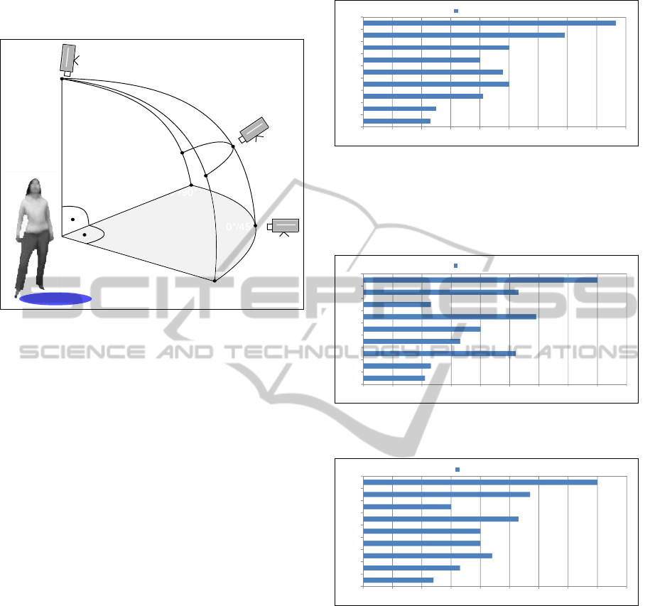
frontal view (total 440 videos in database). Frontal
view videos are assigned by m-fold cross validation.
0°/0°
0°/45°
0°/90°
45°/0°
45°/45°
45°/90°
90°/90°
90°/0°
90°/45°
Figure 6: Illustrating camera angles.
The bar chart in fig. 7 depicts experimental results
for especially recorded video data using directional
informationof image moments. In addition to it AAFI
interval sizes are set to 8.
Videos recorded from a frontal point of view
achieve a maximal accuracy at 0.87. The higher the
horizontal and vertical camera angle, the lower the ac-
curacies. The lowest accuracy is marked at 0.23 for a
90
◦
/90
◦
angle. This behavior is related to the fact,
that the referenced classes contain only videos with
a frontal camera position. In addition a frontal point
of view gives clearer motion. Nevertheless 7 out of
9 camera angles achieve at least an accuracy of 0.40
and the average accuracy is 0.48.
This means our approach works even, if we rotate
the point of view. There are two main reasons for this
observation: First, if the angle is enlarged along just
one axis, motion along the other axis stays almost un-
changed. So for the motion feature vector of one axis
there are little changes. Second, even if the camera
angle changes, the frequency of a movement stays the
same. Only the clearness of the motion direction de-
scends.
Fig. 8 shows experimental results for own video
data using position information of image moments.
Here AAFI interval sizes are set to 4.
Frontally recorded videos result in a maximal ac-
curacy of 0.80. Accuracies for each angle are varying
strongly and the overall accuracy falls to 0.43. The
lowest accuracy measured is 0.21 for a 90
◦
/90
◦
an-
gle. Altogether 5 out of 9 camera angles give an ac-
curacy of at least 0.40. In contrast to directional infor-
mation of moments the position of moments is much
0,40
0,50
0,69
0,87
0,23
0,25
0,41
0,50
0,48
0,00 0,10 0,20 0,30 0,40 0,50 0,60 0,70 0,80 0,90
0°/0°
0°/45°
0°/90°
45°/0°
45°/45°
45°/90°
90°/0°
90°/45°
90°/90°
Accuracy
v/h angle
Figure 7: Accuracies of tests with raw moments and direc-
tional data.
more sensitive to camera angles, because the range of
a movement affects directly the average amplitude of
each frequency interval.
0,59
0,23
0,53
0,80
0,21
0,23
0,52
0,33
0,40
0,00 0,10 0,20 0,30 0,40 0,50 0,60 0,70 0,80 0,90
Accuracy
v/h angle
0°/0°
0°/45°
0°/90°
45°/0°
45°/45°
45°/90°
90°/0°
90°/45°
90°/90°
Figure 8: Accuracies of tests with raw moment positional
data.
0,53
0,30
0,57
0,80
0,24
0,33
0,44
0,40
0,40
0,00 0,10 0,20 0,30 0,40 0,50 0,60 0,70 0,80 0,90
Accuracy
v/h angle
0°/0°
0°/45°
0°/90°
45°/0°
45°/45°
45°/90°
90°/0°
90°/45°
90°/90°
Figure 9: Accuracies of tests with raw moment positional
data and normalized frequency domain.
Settings for tests regarding fig. 9 are the same like
for fig. 8. The only difference is that we normal-
ize here frequency values for classified clips as well
as for referenced clips. Normalization is realized by
dividing each frequency by the frequency maximum
of the whole frequency spectrum. Thereby AAFIs of
classified and referenced clips stay at the same level,
even if the camera angle changes.
Here experimental results do not vary as strong as
in fig. 8 and the average accuracy ascends to 0.45. 6
out of 9 camera angles yield an accuracy about 0.40.
ANALYZING INVARIANCE OF FREQUENCY DOMAIN BASED FEATURES FROM VIDEOS WITH REPEATING
MOTION
663

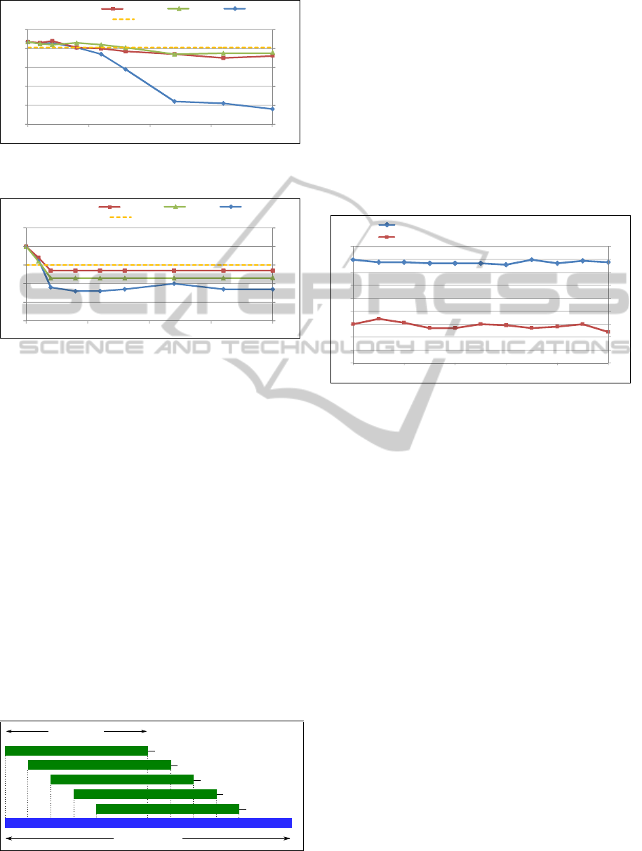
6.3 Scale Invariance
Next two line charts present experimental results for
scale invariance of our approach. The first line chart
shows results for tests with own videos and the sec-
ond line chart regards to external videos. Both in-
ternal and external video sequences are analyzed via
raw moment positions (centroids), since moment di-
rections are always scale invariant. This is related to
the fact that a direction can only be -1, 0 or 1 (see 5).
Scaling has no effect on this values. Experiments are
conducted for 10 different scale factors beginning at
0.25 and ending at 4.0.
Fig. 10 illustrates how accuracies decline when
scaling factor decreases or increases. By decreas-
ing the zooming factor accuracies fall faster than by
zooming in, because the clearness of a motion de-
pends on the range, too. A zooming factor of 1.5
achieves an accuracy of 0.74 and a factor of 0.67
achieves 0.59. For zooming factors 0.5 and 2.5 ac-
curacies stay above 0.30. So the approach works even
for position information of raw moments as far as the
zooming factor is not too high or too low. Normaliz-
ing frequency spectra by maxima or averages of each
spectrum leads to constant accuracies 0.80 and 0.74.
Raw moment directions give a maximal constant ac-
curacy for all scaling factors at 0.87.
0,6
0,7
0,8
0,9
0,1
0,2
0,3
0,4
0,5
0,6
0,25
0,0
0,33
0,4
0,5
0,67
1,0
1,5
2,0
2,5
3,0
4,0
ACC Raw Moment Pos
Avg Norm
Max Norm Pos Direction
zoom factor
0,7
0,8
0,9
0,1
0,2
0,3
0,4
0,5
0,6
1,0
1,0
0,0
Figure 10: Accuracies for internal videos and different
zooming factors.
Now in fig. 11 we see the same effect as in fig.
10. Accuracies decline when scaling factor decreases
or increases. There is just one exception for scaling
factor 1.5. For this factor accuracy increases from
0.40 to 0.42. This behavior is associated with the
referenced classes. External videos are assigned to
own video classes, where distances between camera
and moving object in external clips are bigger than in
own clips. Hence a zoom in aligns external and refer-
enced AAFIs. A normalization of frequency spectra
by maxima or averages of each spectrum results in
constant accuracies 0.32 and 0.28. By utilizing mo-
ment directions the accuracy for each test series stays
at 0.30.
Once again one can see that a zoom out has a
stronger effect on accuracy descend than a zoom in,
because motion ranges become smaller. Here this ef-
fect becomes even more apparent than in fig. 10, be-
cause external videos reveal more irregular motions.
0,00
ACC Raw Moment Pos
Avg Norm
Max Norm Pos Direction
0,25
0,33
0,4
0,5 0,67
1,0 1,5
2,0
2,5
3,0
4,0
zoom factor
0,45
0,40
0,35
0,30
0,25
0,20
0,15
0,10
0,05
0,45
0,40
0,35
0,30
0,25
0,20
0,15
0,10
0,05
0,00
Figure 11: Accuracies for external videos and different
zooming factors.
6.4 Translation Invariance
Varying positions of one activity in different videos
do not influence classification process (translation in-
variance). But shifting motion areas within one video
influences classification process. Next fig. 12 and 13
illustrate how accuracies change in this case. For each
classified clip translation takes place frame by frame.
Further on fig. 12 and 13 plot test results for different
shift directions and shift velocities. Tests with own
videos use directional information of moments and
tests with external videos are performed by position
information.
Fig. 12 visualizes how accuracies for own videos
decrease, when translation velocity is increased. If
vertical or horizontal shift of motion is realized, accu-
racies decrease slightly from 0.87 to 0.75 respectively
0.72. By contrast if diagonal translation is realized
there is a strong decrease from 0.87 to 0.16. The ex-
planation for this different behavior is that shifting a
centroid along just one axis modifies just one coor-
dinate. Unmodified coordinates result in unmodified
features. The yellow line in fig. 12 depicts the ac-
curacy when central moments (variance) are imple-
mented. Here for each translation type and velocity
the accuracy stays always at 0.81.
Next test series in fig. 13 shows that external video
data reacts very sensitive on translation. At the begin-
ning there is a abrupt descent for each curve. Then
horizontal and vertical translation curves stay con-
stantly at 0.27 and 0.23. Accuracy curve for diagonal
shift ends at 0.17. For these abrupt descents two rea-
sons can be stated: One reason is that external videos
depend much more on just one 1D-function than own
videos. Another reason is the greater sensitivity of
positional information of moments to translation than
directional information. Again central moments re-
sult in constant accuracies at 0.30 no matter which
VISAPP 2012 - International Conference on Computer Vision Theory and Applications
664

horizontal
vertical
diagonal
horizontal/vertical/diagonal
Raw Moment Shift
Central Moment Shift
ACC
velocity (pixel/frame)
0,00
0,20
0,40
0,60
0,80
1,00
0,00
0,20
0,40
0,60
0,80
1,00
0
5
10
15
20
Figure 12: Test series with own videos and moments with
translation.
horizontal
vertical
diagonal
horizontal/vertical/diagonal
Raw Moment Shift
Central Moment Shift
velocit

















Figure 13: Test series with external videos and moments
with translation.
translation type or velocity is applied.
Above experiments point out that video sequences
with moving objects or moving cameras can often be
classified more accurate with central moments than
with raw moments. It should be taken into account
that sequences recorded with moving camera need
background subtraction.
6.5 Time Shift Invariance
Now we focus on time shift invariance of AAFIs. In
this context time shift means, that the analyzed video
starts at different points of time. In order to obtain
regular shifts, we use sliding windows with a window
size of 256 frames. The full length of a video is 512
frames. The window is shifted along the time axis
stepwise. After each shift the action inside the sliding
window is classified. Fig. 14 illustrates this idea for a
512 frames long video sequence.
2 Frames
256 Frames
Half Video
Full Video
single shift
double shift
triple shift
quad shift
no shift
.
Figure 14: Time shift illustration.
This technique is used for internal and external
videos during classification stage. Again internal
videos are classified via raw moment directions and
external videos are assigned by raw moment loca-
tions. In fig. 15 it becomes obvious, that the starting
point of a repeating movement has only little effect on
frequency spectra and resulting feature vectors. Here
256 frames of 512 frames long clips are shifted along
the time axis and classified. Each shift has a length of
10 frames. Own videos stay for each shift around an
accuracy level of 0.80 and external videos stay around
0.30. Hence the approach is almost invariant with re-
gard to time shift.
0,1
0,2
0,3
0,4
0,5
0,6
0,7
0,8
0,9
0 20 40 60 80 100
ACC own videos with pos direction
ACC external videos with pos
Frame Shift
0,1
0,2
0,3
0,4
0,5
0,6
0,7
0,8
0,9
0,0
0,0
Figure 15: Accuracies for videos with different starting
times.
7 RELATED RESEARCH
Video annotation and classification can be realized in
many different ways. Main techniques base on key-
frames (Pei and Chen, 2003), texts in frames (Lien-
hart, 1996), audio signals (Patel and Sethi, 1996) and
motions. Each technique has to be robust against dif-
ferent disturbing factors. Focussing on motion and ac-
tion recognition robustness against rotation and trans-
lation is an important task.
Translation invariant methods for human action
classification can be found in (Fanti et al., 2005; Bo-
bick et al., 2001; Niebles and Fei-fei, 2007), where
approaches of Fanti et al. and Bobick et al. also fulfill
scale invariance. A bulk of literature refers to rotation
invariant motion classification. In (Chen et al., 2008)
and (Bashir et al., 2006) rotation invariant methods
for motion trajectory recognition are presented, where
(Chen et al., 2008) provides only planar rotation in-
variance. Results in (Bashir et al., 2006) resemble our
test results, but the maximal number of classes is set
to 5 and the maximal angle size is 60
◦
.
Further on some research work provides methods
with rotation and scale invariance at the same time.
Papers (Weinland et al., 2006; Rao et al., 2003) are
based on Motion History Volumes respectively Mo-
ANALYZING INVARIANCE OF FREQUENCY DOMAIN BASED FEATURES FROM VIDEOS WITH REPEATING
MOTION
665

tion Trajectories, whereas (Abdelkader et al., 2002)
utilizes self-similarity plots resulting from periodic
motion. Unfortunately the research work of Weinland
et al. and Rao et al. do not analyze rotation invari-
ance satisfactorily. The approach of Abdelkader et al.
achieves high accuracies for a wide range of different
camera angles. For a 1-nearest neighbor classifier and
using normalized cross correlation of foreground im-
ages 7 out of 8 angles have an accuracy above 0.60.
A comparison of this work to our work is not possible
due to the fact, that Abdelkader et al. consider only
one class for their classification process.
He and Debrunner compute Hu moments for re-
gions with motion in each frame (He and Debrun-
ner, 2000). Afterwards their system counts the num-
ber of frames until a Hu Moment repeats and define
this number as the motion’s frequency. Hu moments
are invariant for translation, planar rotation, reflection
and scaling. Here the periodic trajectory of an object
cannot be ascertained. A strongly related work to our
approach is given by (Meng et al., 2006). This pa-
per depicts a time shift invariant technique for repeat-
ing movements, but it depends on the MLD-System
(Moving Light Displays).
If we compare our approach to other approaches we
find out, that other approaches do not comprise all dif-
ferent types of invariance as entirely as our method.
8 CONCLUSIONS
In this paper we have shown a scale, view, transla-
tion, reflection and time shift invariant approach for
classifying video sequences. The classification pro-
cess is performed by AAFIs, which represent aver-
age amplitudes of frequency intervals. Frequency
spectra are figured by transforming spatio-temporal
image moment trajectories via FFT. In addition a
novel radius based classifier (RBC) was proposed,
which improved the performance of the system. The
stated accuracies in the experimental phase result
from both selected features and RBC. Other clas-
sifiers (k-nearest neighbor, bayes, average link) we
tested do not achieve same accuracy levels as RBC.
The system’s robustness against different camera
properties (zoom, angle, slide, pan, tilt) is useful for
classifying clips from varying sources. Furthermore it
stays an open issue to adapt and analyze the presented
approach for real time action recognition.
REFERENCES
Abdelkader, C.B., Cutler, R., and Davis, L. (2002). Motion-
based recognition of people in eigengait space. In
Proceedings of the Fifth IEEE Int. Conf. on Automatic
Face and Gesture Recognition, pages 267–277.
Ayyildiz, K. and Conrad, S. (2011). Video classification
by main frequencies of repeating movements. In 12th
International Workshop on Image Analysis for Multi-
media Interactive Services (WIAMIS 2011).
Bashir, F., Khokhar, A., and Schonfeld, D. (2006). View-
invariant motion trajectory-based activity classifica-
tion and recognition. Multimedia Systems, 12(1):45–
54.
Bobick, A. F., Davis, J. W., Society, I. C., and Society, I. C.
(2001). The recognition of human movement using
temporal templates. IEEE Transactions on Pattern
Analysis and Machine Intelligence, 23:257–267.
Chen, X., Schonfeld, D., and Khokhar, A. (2008). Ro-
bust null space representation and sampling for view-
invariant motion trajectory analysis. Computer Vi-
sion and Pattern Recognition, IEEE Computer Society
Conference on, 0:1–6.
Fanti, C., Zelnik-manor, L., and Perona, P. (2005). Hybrid
models for human motion recognition. In IEEE Inter-
national Conf. on Computer Vision, pages 1166–1173.
He, Q. and Debrunner, C. (2000). Individual recognition
from periodic activity using hidden markov models.
In Workshop on Human Motion, pages 47–52.
Lienhart, R. (1996). Indexing and retrieval of digital video
sequences based on automatic text recognition. In
Fourth ACM int. conf. on multimedia, pages 419–420.
Meng, Q., Li, B., and Holstein, H. (2006). Recognition of
human periodic movements from unstructured infor-
mation using a motion-based frequency domain ap-
proach. IVC, pages 795–809.
Niebles, J. C. and Fei-fei, L. (2007). A hierarchical model
of shape and appearance for human action classifica-
tion. In IEEE Computer Society Conference on Com-
puter Vision and Pattern Recognition, pages 1–8.
Patel, N. and Sethi, I. (1996). Audio characterization for
video indexing. In SPIE on Storage and Retrieval for
Still Image and Video Databases, pages 373–384.
Pei, S. and Chen, F. (2003). Semantic scenes detection and
classification in sports videos. In Conf. on Computer
Vision, Graphics and Image Proc., pages 210–217.
Rao, C., Gritai, A., Shah, M., and Syeda-Mahmood, T.
(2003). View-invariant alignment and matching of
video sequences. IEEE International Conference on
Computer Vision, pages 939–945.
Weinland, D., Ronfard, R., and Boyer, E. (2006). Free
viewpoint action recognition using motion history vol-
umes. In Computer vision and image understanding,
pages 249–257.
Wong, W., Siu, W., and Lam, K. (1995). Generation of
moment invariants and their uses for character recog-
nition. Pattern Recognition Letters, 16:115–123.
Zhang, R., Vogler, C., and Metaxas, D. (2004). Human gait
recognition. In Proc. of the 2004 Conf. on Computer
Vision and Pattern Recognition, pages 18–27.
VISAPP 2012 - International Conference on Computer Vision Theory and Applications
666