
SPACE-TIME VISUALIZATION OF DYNAMICS IN LAGRANGIAN
COHERENT STRUCTURES OF TIME-DEPENDENT 2D VECTOR
FIELDS
Sven Bachthaler
1
, Filip Sadlo
1
, Carsten Dachsbacher
2
and Daniel Weiskopf
1
1
VISUS, University of Stuttgart, Stuttgart, Germany
2
Karlsruhe Institute of Technology, Karlsruhe, Germany
Keywords:
Flow Visualization, Lagrangian Coherent Structures, Hyperbolic Trajectories.
Abstract:
Lagrangian coherent structures (LCS), apparent as ridges in the finite-time Lyapunov exponent (FTLE) field,
represent a time-dependent alternative to the concept of separatrices in vector field topology. Traditionally,
LCS are analyzed and visualized in terms of their geometric shape only, neglecting stretching and compression
in tangent directions. These effects are, however, of particular interest in mixing phenomena and turbulence.
Hyperbolicity plays an important role in these processes and gives rise to hyperbolic trajectories originating at
the intersections of forward and reverse LCS. Since integration of hyperbolic trajectories is difficult, we pro-
pose to visualize the corresponding space-time intersection curves of LCS instead. By stacking the traditional
2D FTLE video frames of time-dependent vector fields, a space-time FTLE field is obtained. In this field, ridge
lines turn into ridge surfaces representing LCS, and their intersection forms curves that are a robust alterna-
tive to hyperbolic trajectories. Additionally, we use a space-time representation of the time-dependent vector
field, leading to a steady 3D space-time vector field. In this field, the LCS become stream surfaces given that
their advection property is sufficiently met. This makes visualization of the dynamics within LCS amenable
to line integral convolution (LIC), conveying in particular the dynamics around hyperbolic trajectories. To
avoid occlusion, the LCS can be constrained to space-time bands around the intersection curves, resembling
visualization by saddle connectors. We evaluate our approach using synthetic, simulated, and measured vector
fields.
1 INTRODUCTION
As science and engineering methods evolve, model-
ing of phenomena is shifting from stationary to time-
dependent domains. 2D computational fluid dynam-
ics (CFD) simulations are of major importance in sev-
eral domains, such as the analysis of flow in films and
on free-slip boundaries. To examine and understand
such data, efficient tools for analysis and visualization
are required. Feature extraction techniques, provid-
ing a condensed representation of the essential infor-
mation, are often applied to the visualization of vec-
tor fields. A prominent concept revealing the overall
structure is vector field topology (Helman and Hes-
selink, 1989). Whereas vector field topology is di-
rectly applicable only to steady or quasi-stationary
vector fields, Lagrangian coherent structures (LCS)
(Haller, 2001) are popular for the analysis of time-
dependent vector fields. LCS are a time-dependent
counterpart to separatrices, which are streamlines st-
arted from separating regions of different behavior.
LCS have been increasingly subject to research in
the last decade and can be obtained as maximizing
curves (ridges) in the finite-time Lyapunov exponent
(FTLE), a scalar field measuring the separation of tra-
jectories (Haller, 2001). FTLE computation is, how-
ever, an expensive task because at least one trajectory
needs to be computed per sample point. LCS behave
as material lines under the action of time-dependent
flow, i.e., they are advected and exhibit negligible
cross-flow for sufficiently long advection time inter-
vals, as reported by Haller (Haller, 2001), Lekien et
al. (Lekien et al., 2005), and Sadlo et al. (Sadlo et al.,
2012). This property gives rise, e.g., to the acceler-
ation technique by Sadlo et al. (Sadlo et al., 2011)
based on grid advection.
Our new method adopts the concept of hyperbolic
trajectories and space-time streak manifolds, which
we therefore discuss in the following. Previous work
by Sadlo and Weiskopf (Sadlo and Weiskopf, 2010)
573
Bachthaler S., Sadlo F., Dachsbacher C. and Weiskopf D..
SPACE-TIME VISUALIZATION OF DYNAMICS IN LAGRANGIAN COHERENT STRUCTURES OF TIME-DEPENDENT 2D VECTOR FIELDS.
DOI: 10.5220/0003810905730583
In Proceedings of the International Conference on Computer Graphics Theory and Applications (IVAPP-2012), pages 573-583
ISBN: 978-989-8565-02-0
Copyright
c
2012 SCITEPRESS (Science and Technology Publications, Lda.)
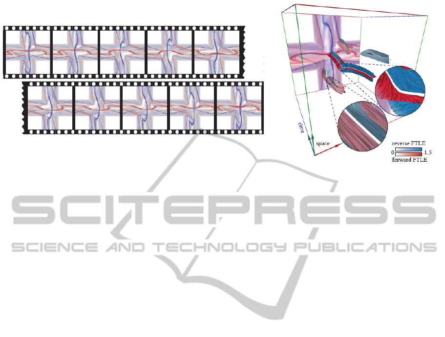
Figure 1: Left: traditional visualization of a time-dependent vector field by time series of the finite-time Lyapunov exponent
is difficult to analyze and does not convey the dynamics inside its ridges (Lagrangian coherent structures). Right: our space-
time representation reveals the overall structure and makes the dynamics inside the Lagrangian coherent structures visible by
line texture patterns. Close-ups: in contrast to the traditional 2D visualization, different dynamics along intersection curves
(almost parallel flow on the left vs. strongly hyperbolic flow on the right) is apparent.
generalized vector field topology to time-dependent
vector fields by replacing the role of streamlines by
generalized streak lines (Wiebel et al., 2007). This
way, critical points turn into degenerate streak lines
and separatrices into streak lines (space-time streak
manifolds) converging toward these degenerate streak
lines in forward or reverse time. It was found that
these need to be distinguished degenerate streak lines
identical to the previously discovered hyperbolic tra-
jectories (Haller, 2000).
Hyperbolic trajectories can be seen as constituent
structures in time-dependent 2D vector field topol-
ogy. As mentioned, space-time streak manifolds—
the time-dependent counterpart to separatrices—can
be constructed alone from hyperbolic trajectories—
no dense sampling is required in contrast to the FTLE
approach. However, a major limitation with hyper-
bolic trajectories is the difficulty of their integration.
Although the integration error tends to grow exponen-
tially in linear vector fields, it is usually negligible due
to comparably short advection times and low separa-
tion rates along common trajectories. Unfortunately,
this is not the case in typical hyperbolic configura-
tions due to large separation rates and the fact that
both forward and reverse integration are subject to re-
pulsion from one of the LCS (see Fig. 2). Hyperbolic
trajectories coincide with the intersection of forward
and reverse LCS; since ridges in forward FTLE repre-
sent repelling LCS whereas those in reverse FTLE are
attracting, the trajectory is repelled from the former
forward and from the latter in backward direction.
Our method has therefore a twofold objective:
(1) avoiding the integration of hyperbolic trajecto-
ries by replacing them with intersections of LCS, and
(2) revealing tangential dynamics in LCS, accom-
plished by line integral convolution (LIC). By treat-
ing time as an additional dimension, we obtain a sta-
tionary visualization that conveys the overall struc-
ture in space-time. Several approaches for obtaining
seeds for hyperbolic trajectories exist: by intersecting
ridges in hyperbolicity time (Haller, 2000), ridges in
FTLE (Sadlo and Weiskopf, 2010), and constructing
streak manifolds from them, or by building a time-
dependent linear model from critical points (Ide et al.,
2002). This kind of visualization of hyperbolic tra-
jectories is, however, restricted to LCS geometry, i.e.,
the dynamics in the vicinity of the hyperbolic trajecto-
ries is not conveyed. Furthermore, the hyperbolicity
of the vector field is typically analyzed by requiring
negative determinant of the velocity gradient. This
approach fails in providing insight into the role and
importance of hyperbolic trajectories. In contrast, our
LIC-based visualization captures the configuration of
the flow in the neighborhood of hyperbolic trajecto-
ries and also in general along LCS. One example is
the discrimination of almost parallel flow configura-
tions from strongly hyperbolic ones (Fig. 1, (right)).
This provides increased insight in the overall dynam-
ics, interplay, and importance of LCS. For example,
this allows for a qualitative analysis of mixing phe-
nomena. We refer the reader to fluid mechanics litera-
ture, e.g., (Mathur et al., 2007) for the underlying con-
cepts, e.g., for details on mixing and the Lagrangian
skeleton of turbulence.
IVAPP 2012 - International Conference on Information Visualization Theory and Applications
574
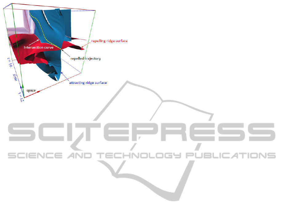
Figure 2: Space-time ridge surfaces in forward (red) and
reverse (blue) finite-time Lyapunov exponent together with
cross section at final time step (colored). The space-time
intersection curve in the center (white) represents a hyper-
bolic trajectory. Traditional integration of the hyperbolic
trajectory from the initial intersection is difficult due to ex-
ponential growth of error (yellow curve).
2 RELATED WORK
Work that is closely related to our objectives was dis-
cussed in the previous section, here we give a short
overview of work that is in weaker context.
Many applications of vector field topology in fluid
mechanics have been presented by Perry et al. (Perry
and Chong, 1987). It was later introduced in visual-
ization by Helman and Hesselink (Helman and Hes-
selink, 1989), (Helman and Hesselink, 1991) again in
the context of flow fields. For details, we refer the
reader to the work by Globus et al. (Globus et al.,
1991), Asimov (Asimov, 1993), and Abraham and
Shaw (Abraham and Shaw, 1992).
Vector field topology did also give rise to derived
concepts and techniques. Examples are saddle con-
nectors (Theisel et al., 2003) and boundary switch
curves (Weinkauf et al., 2004a), both augmenting vec-
tor field topology by line-type features. Several ap-
proaches have been proposed for adopting the con-
cepts to time-dependent vector fields, including the
path line oriented topologies for 2D vector fields by
Theisel et al. (Theisel et al., 2004) and Shi et al. (Shi
et al., 2006), Galilean-invariant alternatives for criti-
cal points (Kasten et al., 2010), and basics for a La-
grangian vector field topology (Fuchs et al., 2010).
Separatrices and LCS are able to convey the struc-
tural and temporal organization of vector fields, how-
ever, at the same time, they suffer from this prop-
erty; vector direction and magnitude are not repre-
sented, neither along these constructs, nor, and more
importantly, in their vicinity. There are different
approaches to overcome these drawbacks. Critical
points are often visualized with glyphs representing
the linearized flow. Another approach is to augment
separatrices with arrows as presented by Weinkauf et
al. (Weinkauf et al., 2004b). However, the most com-
mon approach in 2D and 3D vector field topology is
to combine the separatrices with line integral convolu-
tion (LIC), e.g., see Weiskopf and Ertl (Weiskopf and
Ertl, 2004). This vector field visualization with LIC
can be either drawn between separatrices in the case
of 2D vector fields, or on the separatrices themselves
in the case of 3D vector fields. For time-dependent
vector fields, this approach is not applicable because
LIC visualizes transport along streamlines, i.e., in-
stantaneous field lines, whereas LCS are usually ob-
tained using true trajectories, i.e., from path lines.
Therefore, other methods are required for visualiz-
ing the advection in the context of LCS, e.g., Shad-
den et al. (Shadden et al., 2005) advect particles. We
exploit the fact that 2D time-dependent vector fields
can be turned into 3D stationary vector fields by di-
mension lifting. Since the resulting domain is steady,
streamlines are then equal to path lines, which allows
us to use LIC. Texture-based methods (like LIC) have
the advantage of avoiding the seed point positioning
problem by conveying the field structure in a dense
fashion. Since there is no intrinsic, predefined sur-
face parametrization available, image-space oriented
methods like (Laramee et al., 2003), (Wijk, 2003),
and (Weiskopf and Ertl, 2004) are predestined for our
task (we build on the latter one). More background in-
formation on texture-based vector field visualization
can be found in the survey of (Laramee et al., 2004).
3 SPACE-TIME LCS
VISUALIZATION
Our new visualization technique builds on the fact
that time-dependent vector fields can be turned into
stationary ones by treating time as additional dimen-
sion. This approach is common in the field of dif-
ferential equations, where non-autonomous systems
are made autonomous. Hence, 2D time-dependent
vector fields (u(x,y,t),v(x,y,t))
>
are converted into
steady 3D vector fields (u(x,y,t),v(x,y,t),1)
>
, which
we denote as space-time vector fields. All fol-
lowing steps of our algorithm (see Fig. 4) take
place in this space-time domain. Since 2D path
lines represent streamlines in space-time, we use
3D streamline integration over advection time T in-
side the space-time vector field to generate a flow
map φ(x,y,t) 7→ (x
0
,y
0
,t + T )
>
. Then, for each time
SPACE-TIME VISUALIZATION OF DYNAMICS IN LAGRANGIAN COHERENT STRUCTURES OF
TIME-DEPENDENT 2D VECTOR FIELDS
575
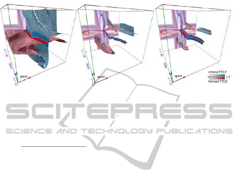
(a) (b) (c)
Figure 3: Building blocks for space-time LCS visualization, shown with the example from Sec. 5.1. Advection time for
forward and reverse FTLE is T = 4s. (a) Space-time LIC qualitatively visualizes LCS dynamics: hyperbolic behavior is
apparent. In addition, hyperbolicity is encoded by color saturation. A minimum FTLE value of 0.5 is used. (b) Intersection
bands by clipping with complementary FTLE reduce occlusion but still provide context and convey structure of reverse
FTLE. The minimum complementary FTLE value is 0.41. (c) Intersection bands by clipping with distance to intersection
curves further reduces occlusion and provides the topological skeleton.
slice
¯
t of the space-time stack we compute the tradi-
tional 2D FTLE according to Haller (Haller, 2001) as
1/|T | ln
p
λ
max
[(∇
2
φ(x,y,
¯
t))
>
∇
2
φ(x,y,
¯
t)] with ∇
2
=
(∂/∂x,∂/∂y,0)
>
and major eigenvalue λ
max
(·). LCS
are then extracted from the resulting stack of tradi-
tional 2D FTLE fields by ridge surface extraction, dis-
cussed in Section 3.1.
Due to the discussed material advection property
of LCS, these surfaces represent stream surfaces in
the space-time vector field, i.e., they are tangent to the
space-time flow. This allows a direct application of
LIC techniques, which we describe in Section 3.3. By
this, LIC visualizes the dynamics of path lines along
which the LCS are advected, and hence the dynamics
within the LCS. As intersections of stream surfaces
are streamlines, the space-time intersection of these
LCS surfaces from forward and reverse FTLE repre-
sents a counterpart to hyperbolic trajectories. In Sec-
tion 3.2, we address the investigation of these inter-
section curves in terms of hyperbolicity, again based
on LCS. Restricting the LIC visualization to bands
around the intersection curves comprises our second
major contribution, detailed in Section 3.4.
3.1 Ridge Surface Extraction
We extract the ridge surfaces from the stack of 2D
FTLE fields as height ridges (Eberly, 1996) of codi-
mension one from the 3D space-time FTLE field,
according to Sadlo and Peikert (Sadlo and Peikert,
2009). We follow this approach to avoid the prob-
lems that would arise from stitching of the individual
ridge curves from the 2D FTLE fields. Furthermore,
ridges are typically non-manifold, which would cause
further issues. Since Eberly’s formulation (Eberly,
1996) is local and relies on higher-order derivatives, it
is subject to erroneous solutions. It is therefore com-
mon practice to apply filtering and we follow the fil-
tering process described by Sadlo and Peikert (Sadlo
and Peikert, 2007): since only sufficiently “sharp”
FTLE ridges represent LCS, ridge regions where the
modulus of the eigenvalue of the Hessian is too low
are suppressed. Further, we require a minimum FTLE
value, hence requiring a minimum separation strength
of the LCS. Finally, to suppress small ridges, we fil-
ter the ridge surfaces by area. As described in (Sadlo
and Peikert, 2007), we also use a least-squares ap-
proach to prevent noise amplification during estima-
tion of the gradient and Hessian. Figure 2 shows ex-
amples of ridges extracted from a stack of forward
and reverse-time FTLE: repelling LCS (ridges in for-
ward FTLE) colored red and attracting ones (ridges
in reverse FTLE) blue. The space-time structure of
the field is revealed including the intersection curves.
However, this does not convey hyperbolicity aspects,
e.g., it does not disambiguate intersection curves rep-
resenting strong hyperbolic trajectories from weak
hyperbolic ones. This motivates the visualization of
hyperbolicity on LCS.
3.2 Visualizing Hyperbolicity
To help the user in the investigation of hyper-
bolic effects, and hyperbolic trajectories in partic-
IVAPP 2012 - International Conference on Information Visualization Theory and Applications
576

ular, we map hyperbolicity to saturation, shown in
Fig. 3a. We have chosen the hyperbolicity definition
by Haller (Haller, 2000), i.e., the sign of the determi-
nant of the velocity gradient of the original 2D vec-
tor field at the respective space-time location. One
can see how this technique not only reveals the pres-
ence of hyperbolicity but also allows for the interpre-
tation of the hyperbolic regions around the intersec-
tion curves. To examine hyperbolicity more precisely,
we introduce a novel technique to visualize LCS dy-
namics in the next section.
3.3 Visualizing LCS Dynamics
The LCS in our space-time FTLE field are present as
ridge surfaces and to fully capture the spatial varia-
tion of their dynamics they lend themselves to dense
texture-based visualization such as LIC. Since LCS
lack intrinsic surface parametrization and need to be
analyzed in overview scales as well as in local detail,
image-space oriented approaches are predestined to
visualize the space-time structure. We use the hybrid
physical/device-space LIC approach by Weiskopf and
Ertl (Weiskopf and Ertl, 2004), which relies on par-
ticle tracing computed in the physical space of the
object and in the device space of the image plane at
the same time. The LIC pattern is based on the tan-
gential part of the vectors attached to our surfaces.
This dual-space approach combines the advantages of
image-space methods with frame-to-frame coherence
and avoids inflow issues at silhouette lines. For a de-
tailed description of this visualization technique, we
refer to the original paper.
In the context of our visualization of LCS dynam-
ics, the goal is to visualize the space-time direction
of the vector field. Hence, we normalize the space-
time vectors during LIC computation to obtain LIC
line patterns of uniform length for optimal perception.
In contrast to traditional spatial LIC, we retain the vi-
sual encoding of velocity magnitude in the form of
surface orientation in space-time. For example, small
angles between surface normal and the time axis indi-
cate high speed.
Figure 3a exemplifies the method again on the
same data set. It is apparent how this technique con-
veys the time-dependent dynamics within LCS. Com-
bining it with the saturation-based visualization of hy-
perbolicity (Section 3.2) supports the identification of
hyperbolic intersection curves and still provides the
LCS dynamics context. Since LCS are often convo-
luted, they typically exhibit many intersections that
are, however, often occluded. We address this prob-
lem by the building block described next: the restric-
tion of the technique to regions around space-time
LCS intersection curves. At the same time, this ap-
proach explicitly addresses the analysis of the inter-
section curves.
3.4 LCS Intersection Bands
Even in the simple example shown so far, it is obvi-
ous that occlusion tends to be a problem in space-time
visualization of LCS. To address this and to provide
a method for analyzing intersection curves of LCS
at the same time, we introduce two complementary
approaches that have proven valuable in our experi-
ments, both restricting the presented visualization to
bands around the LCS intersection curves.
As discussed in Section 3.1, a common approach
is to filter FTLE ridges by prescribing a minimum
FTLE value. This way, the visualization is restricted
to important LCS, i.e., those representing strong sep-
aration. This filter is applied to ridges in both forward
and reverse FTLE fields. If we additionally prescribe
a minimum value for the complementary FTLE, i.e.,
the reverse in case of forward FTLE ridges and the
forward in case of reverse FTLE ridges, one typically
restricts the visualization to bands around the inter-
section curves, shown in Fig. 3b. This technique has
the advantage that the profile of the complementary
FTLE field is conveyed, allowing qualitative interpre-
tation of the interplay of LCS. Furthermore, it often
features additional bands that do not exhibit LCS in-
tersections. They are generated if FTLE ridges are lo-
cated in regions of high complementary FTLE. These
additional bands are still of interest: the respective
regions exhibit both high forward and reverse-time
FTLE. Additionally, these bands may connect to other
bands that feature intersection curves and hence con-
vey the overall organization of the LCS. A drawback
of this approach, however, is that the bands may get
too narrow for appropriate LIC visualization or too
wide to sufficiently reduce occlusion.
Therefore, we propose, as an alternative, to re-
strict the LCS to the neighborhood of their intersec-
tion curves. To avoid numerical issues, we first omit
regions where the LCS intersect at small angle.
Furthermore, a minimum length of the intersec-
tion curves is required to obtain significant visual-
izations. The remaining intersection curves are then
used for distance computation, leading to a distance
field on the LCS that is then used for clipping. Fig-
ure 3c shows an example: the dynamics of the LCS is
well depicted by LIC and at the same time occlusion
is substantially reduced, allowing for the analysis of
the intersection curves with respect to LCS dynamics
and hyperbolicity. Since the resulting bands can still
be too narrow due to perspective foreshortening, we
SPACE-TIME VISUALIZATION OF DYNAMICS IN LAGRANGIAN COHERENT STRUCTURES OF
TIME-DEPENDENT 2D VECTOR FIELDS
577
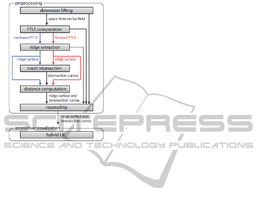
Figure 4: Overview of our technique, accompanied by the
data that are passed between the stages of the pipeline.
also support depth-corrected width of the bands de-
scribed in Section 4.2.
To sum up, these clipping approaches result in vi-
sualizations that can be seen as an extended topologi-
cal skeleton of time-dependent flow. Note that we use
equal thresholds for forward and reverse-time FTLE
ridge filtering as well as for complementary FTLE
band clipping, for ensuring consistent visualization.
Finally, we would like to point out the similarity to
saddle connectors (Theisel et al., 2003), although our
approach resides in space-time, whereas saddle con-
nectors visualize 3D steady vector fields.
3.5 Combined Visualization
Our system allows the user to interactively switch on
and off the clipping for intersection bands. When
clipping is enabled, the remaining choice is between
complementary FTLE and distance-based intersec-
tion bands. Depth-correction of intersection band
width is always enabled. In summary, only three dif-
ferent modes (no clipping, complementary clipping,
distance-based clipping) are required to cover the vi-
sualization needs.
4 IMPLEMENTATION
This section details the implementation of the differ-
ent building blocks of our technique as well as modifi-
cations to existing approaches. The pipeline shown in
Fig. 4 gives an overview of the steps and provides in-
formation about the data that are exchanged between
different stages of the pipeline.
4.1 Preprocessing
Several steps in our technique are performed in a pre-
processing phase, once per data set.
The original data set is given as a series of time
steps of a 2D vector field. To create the stationary
space-time 3D vector field, we apply dimension lift-
ing, i.e., the time series of the 2D vector field are
stacked and the time dimension is treated as addi-
tional third dimension. This space-time vector field
is used to compute the 3D space-time FTLE field for
forward and reverse time direction. Using this FTLE
field, ridge surfaces are extracted. A detailed descrip-
tion of the ridge extraction method is given by Sadlo
and Peikert (Sadlo and Peikert, 2007).
The ridge surface meshes from forward and
reverse–time FTLE are intersected to obtain the in-
tersection curves. Once the geometry of all intersec-
tion curves is obtained, a distance field is computed
that holds the distance of ridge surface vertices to the
nearest intersection curve. Next, we compute vertex-
based normals, which are used for shading in the in-
teractive visualization. During this process, normals
are reoriented if necessary; however, since ridge sur-
faces are not necessarily orientable, we may not suc-
ceed for all normals. Remaining inconsistencies for
the normals are treated during interactive visualiza-
tion using a shader. Finally, the space-time flow vec-
tors are sampled at the vertex locations of the ridge
surface mesh. This resampling is independent of the
FTLE sampling grid, allowing for acceleration meth-
ods (Garth et al., 2007), (Sadlo and Peikert, 2007),
and (Hlawatsch et al., 2011). Distance values, nor-
mals, resampled flow vectors, and additional scalars
like FTLE values, hyperbolicity, and the minor eigen-
value of the Hessian (see Section 3.1) are attached to
the ridge surface mesh that is then passed to the inter-
active visualization stage.
4.2 Interactive Visualization
The core of our interactive visualization is based on
hybrid physical/device-space LIC (Weiskopf and Ertl,
2004) to create line-like texture on the ridge surfaces.
During rendering of the space-time ridge surfaces,
we apply Phong illumination to enhance visibility and
perception of the geometry. Since the ridge surfaces
may be non-orientable, we have to ensure that local
IVAPP 2012 - International Conference on Information Visualization Theory and Applications
578

normal vectors are consistently oriented in order to
avoid shading artifacts. Therefore, we make normal
orientation consistent during fragment processing us-
ing the dot product between normal and view vec-
tor. This prevents inconsistent shading due to nor-
mal interpolation; however, ridge surfaces may still
appear rippled. This happens because of FTLE alias-
ing effects at strong and sharp ridges, where very
high FTLE gradients are present. To compensate for
this, we correct the normals to be perpendicular to the
space-time vector field and hence to its LCS during
fragment processing.
We handle occlusion by attaching additional data
(regular FTLE, complementary FTLE, distance to
nearest intersection curve) obtained during the pre-
processing stage (see Section 4.1) to each vertex of
the ridge surface mesh and upload this data as ad-
ditional texture coordinates to the GPU. Fragments
that do not meet the filtering criteria are discarded.
All thresholds used in this process are adjustable in
real-time by the user. In addition to user controlled
clipping, we adjust the width of our LCS intersection
bands if they are clipped by the distance to the nearest
intersection curve. We adjust the clipping threshold
based on distance to the camera position. This re-
sults in intersection bands with constant image-space
width, which reduces occlusion of intersection bands
that are close to the camera. At the same time, in-
tersection bands that are farther away are enlarged,
which improves visibility of the LIC pattern.
5 RESULTS
We apply the presented methods to different data sets.
The first two data sets are synthetic, whereas the third
is created by CFD simulation, and the fourth is ob-
tained by remote sensing of ocean currents.
Our implementation was tested on a PC with an
Intel Core Quad CPU (2.4 GHz), 4 GB of RAM and
an NVIDIA GeForce 275 GPU with 896 MB of ded-
icated graphics memory. Each of the presented data
sets is visualized at interactive rates. Since our im-
plementation is based on the approach presented by
Weiskopf and Ertl (Weiskopf and Ertl, 2004), it shows
the same performance behavior—we refer to their pa-
per for a detailed performance analysis.
A bounding box of the domain helps the user to
navigate and orientate in space-time. This bounding
box is color coded—the time dimension is indicated
by a blue axis while the two spatial dimensions have a
red and green axis, respectively. The last time step of
the space-time region of interest is located at the back
end of the bounding box which shows the FTLE field
(a) (b)
Figure 5: (a) Gyre Saddle example at t = 0. (b) Quad Gyre
example at t = 0.
as a color–coded texture. In this texture, FTLE values
are mapped to saturation, with full saturation mapping
to the highest FTLE value. There, we use the same
color-coding as for the space-time ridge surfaces.
5.1 Oscillating Gyre Saddle
The synthetic vector field that we use as an example
in this section is due to Sadlo and Weiskopf (Sadlo
and Weiskopf, 2010). It exhibits a non-linear sad-
dle (Fig. 5a) that oscillates between the locations
(0.25,0.25) and (−0.25, −0.25) at a period of τ = 4.
Please refer to Fig. 1, Fig. 2, and Fig. 3 for resulting
visualizations. To sum up, it exhibits a strongly hy-
perbolic intersection curve visualized in Fig. 1 (right)
and several non-hyperbolic ones. This is consistent
with the Eulerian picture (Fig. 5a) showing distin-
guished saddle behavior at its center. As mentioned
by Sadlo and Weiskopf (Sadlo and Weiskopf, 2010),
there are other ridges due to shear processes. These
are of inferior importance for mixing and cannot give
rise to hyperbolic trajectories, i.e., their LIC patterns
do not show hyperbolic behavior. Note that we filter
FTLE ridges to show the strongest and largest LCS.
Supressing weaker ridges simplifies the resulting vi-
sualization which we use for depicting purposes.
(a) (b) (c)
Figure 6: Three time steps of the buoyant plume exam-
ple, color indicates temperature (red maps to high temper-
ature, blue to low temperature). (a) Two plumes build up
and travel toward each other in vertical direction. (b) After
collision, two new plumes are created that travel toward the
walls. (c) After collision with the side walls.
SPACE-TIME VISUALIZATION OF DYNAMICS IN LAGRANGIAN COHERENT STRUCTURES OF
TIME-DEPENDENT 2D VECTOR FIELDS
579
(a) (b) (c)
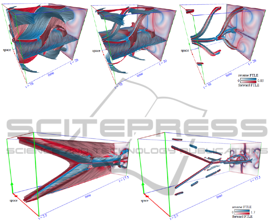
Figure 7: Quad-Gyre example. The advection time for forward and reverse FTLE is T = 7.5s. (a) Full visualization of
forward and reverse LCS. A lower FTLE threshold of 0.4 is used. (b) Visualization restricted to complementary FTLE bands.
Minor artifacts appear due to aliasing effects of forward and reverse FTLE. The minimum complementary FTLE value is
0.19. (c) Restriction to distance-based LCS intersection bands reveals the topological space-time skeleton.
(a) (b)
Figure 8: Buoyant plumes example. The advection time for forward and reverse FTLE is T = 1.5s. (a) Full visualization of
forward and reverse LCS. The dynamics of the two plumes is apparent in the first part of the examined time interval. A lower
FTLE threshold of 0.87 is used. (b) LCS intersection bands clipped by distance, revealing the skeleton.
5.2 Quad Gyre
The double gyre example was introduced by Shad-
den et al. (Shadden et al., 2005) to examine FTLE
and LCS, and to compare them to vector field topol-
ogy. It consists of two vortical regions separated by a
straight separatrix that connects two saddle-type crit-
ical points: one oscillating horizontally at the upper
edge and the other synchronously oscillating horizon-
tally along the lower edge. This is a prominent ex-
ample where the vector field topology result substan-
tially differs from LCS. This data set is temporally
periodic. To avoid boundary issues, we use a larger
range of field, resulting in four gyres. As proposed
by Shadden et al., we use the configuration ε = 1/4,
ω = π/5, and A = 1/10. Figure 5b shows a plot at
t = 0 for these parameters.
Rendering the quad gyre without clipping (Fig. 7a)
results in space-time ridges that heavily occlude each
other. Please note that the y = 0 plane represents an
LCS in both forward and reverse direction, which re-
sults in z-fighting. Nevertheless, the LIC line pattern
is consistent in that region due to the image-based
LIC technique. Reducing occlusion by clipping with
the complementary FTLE (Fig. 7b) removes parts of
the ridge surfaces, while preserving the context of the
bands. Note, for example, that the red bands are con-
nected at the upper edge of the domain and hence
are part of the same LCS. If we clip the space-time
ridge surfaces by distance to their intersection curves
(Fig. 7c), occlusion is even more reduced, but less
context is conveyed. However, this technique espe-
cially pays off in data sets with complex space-time
dynamics, since the topological skeleton is well visi-
IVAPP 2012 - International Conference on Information Visualization Theory and Applications
580
(a) (b)
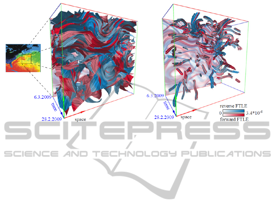
Figure 9: OSCAR example. The advection time for forward and reverse FTLE is T = 25 days. The small map on the left
hand side shows the atlantic ocean and the east coast of North America. It gives a frame of reference for our visualization
results and exemplifies the prevalent mixing due to the gulf stream. Please note that this map does not show flow but rather
water temperature mapped to colors and that it was generated outside of the investigated time interval. (a) Full visualization
of forward and reverse LCS. A lower FTLE threshold of 9 × 10
−7
is used. Flow around several intersection curves shows
strong hyperbolic behavior. (b) LCS intersection bands clipped by distance.
ble from most views. In all images, hyperbolicity is
visualized by mapping it to the saturation of the ridge
surface color. It can be seen that it readily guides at-
tention to hyperbolic LIC patterns. As in the results
by Sadlo and Weiskopf (Sadlo and Weiskopf, 2010),
we identify a hyperbolic trajectory at the center of the
data set.
5.3 Buoyant Plumes
This data was obtained by a CFD simulation of buoy-
ant 2D flow. A square container was modeled with
a small heated region at its bottom wall and a small
cooled region at its top wall. Figure 6 illustrates the
flow. Two plumes are developed, a hot one rising to
the top and a cold one moving in reverse direction to
the bottom. They then collide at the center and give
rise to two new plumes traveling horizontally toward
the side walls. As they approach the walls, they both
split and produce plumes traveling in vertical direc-
tion. From that point on, the regular behavior is re-
placed by increasingly turbulent flow behavior.
Figure 8a shows the visualization of both forward-
and reverse-time FTLE ridges. There is no clipping
applied for this image but saturation already guides
to the hyperbolic regions, however, many of them are
occluded. In Fig. 8b, the distance-based LCS inter-
section bands nicely visualize the hyperbolic mech-
anisms. One can see how the two plumes approach
each other and merge, then divide and later give rise
to turbulent flow. We finally identify several strong
hyperbolic regions toward the end of the examined
time interval. The multitude of hyperbolic regions ap-
proves the observation of strong buoyant mixing. The
high intricacy and topological complexity of turbulent
buoyant flow reflects in our visualization.
5.4 OSCAR
Ocean Surface Currents Analyses Real-time (OS-
CAR) (Bonjean and Lagerloef, 2002) is a project to
calculate ocean surface velocities from satellite data.
The OSCAR product is a direct computation of global
surface currents using satellite sea surface height,
wind, and temperature. The OSCAR analyses have
been used extensively in climate studies, such as for
ocean heat storage and phytoplankton blooms.
We applied our technique to the gulf stream at
the east coast of North America. We thereby focused
on a strong hyperbolic LCS system involved in mix-
ing (Fig. 9a). As expected, our technique revealed a
complex Lagrangian skeleton of turbulence (Mathur
et al., 2007), shown in Fig. 9a. Our LIC patterns
allow a direct and qualitative inspection of the LCS
with respect to hyperbolic mechanisms and mixing.
Whereas many regions in the OSCAR data set ex-
hibited inferior hyperbolic behavior, it is prominent
in the selected region. Again, the LCS intersection
SPACE-TIME VISUALIZATION OF DYNAMICS IN LAGRANGIAN COHERENT STRUCTURES OF
TIME-DEPENDENT 2D VECTOR FIELDS
581

bands dramatically reduce occlusion while still con-
veying topological structure and hyperbolic dynam-
ics, see Fig. 9b. Following the LIC line patterns along
the temporal axis directly conveys the action of the
flow in terms of mixing, i.e., thinning and folding.
6 CONCLUSIONS
We have presented an approach for the visualiza-
tion and analysis of the dynamics in LCS of time-
dependent 2D vector fields. Compared to traditional
approaches, we do not restrict the investigation of
LCS to their geometric shape. We extend the visu-
alization by allowing the user to analyze the intrin-
sic dynamics of LCS in terms of stretching and com-
pression, in particular along hyperbolic trajectories.
These dynamics are visualized by space-time LIC on
space-time ridge surfaces of the 2D FTLE.
Occlusion problems due to convoluted and heav-
ily intersecting LCS are reduced by clipping of the
LCS, providing LCS intersection bands. Clipping can
be based on the distance to the hyperbolic trajecto-
ries and on forward and reverse FTLE to suppress less
important regions. A major numerical aspect of our
method is the avoidance of the difficult direct inte-
gration of hyperbolic trajectories, we intersect FTLE
ridge space-time surfaces instead. Still, the growth
of the respective space-time streak manifolds is con-
veyed by the LIC.
Finally, we have demonstrated the applicability of
our method with several synthetic and real-world data
sets, also in the context of turbulent flow analysis, a
topic of ongoing research. In future work, we plan
to extend our technique to 3D time-dependent vector
fields, i.e., investigate intersection curves of LCS and
the surfaces they span over time.
ACKNOWLEDGEMENTS
The first author and fourth author thank the Ger-
man Research Foundation (DFG) for financial sup-
port within SFB 716 / D.5 at University of Stuttgart.
The second author thanks DFG for financial support
within the Cluster of Excellence in Simulation Tech-
nology (EXC 310/1), and SFB-TRR 75 at University
of Stuttgart.
REFERENCES
Abraham, R. H. and Shaw, C. D. (1992). Dynamics, the
Geometry of Behavior. 2nd ed. Addison-Wesley.
Asimov, D. (1993). Notes on the topology of vector fields
and flows. Technical Report RNR-93-003, NASA
Ames Research Center.
Bonjean, F. and Lagerloef, G. (2002). Diagnostic model
and analysis of the surface currents in the tropical
pacific ocean. Journal of Physical Oceanography,
32(10):2938–2954.
Eberly, D. (1996). Ridges in Image and Data Analysis.
Computational Imaging and Vision. Kluwer Aca-
demic Publishers.
Fuchs, R., Kemmler, J., Schindler, B., Sadlo, F., Hauser,
H., and Peikert, R. (2010). Toward a Lagrangian
vector field topology. Computer Graphics Forum,
29(3):1163–1172.
Garth, C., Gerhardt, F., Tricoche, X., and Hagen, H.
(2007). Efficient computation and visualization of
coherent structures in fluid flow applications. IEEE
Transactions on Visualization and Computer Graph-
ics, 13(6):1464–1471.
Globus, A., Levit, C., and Lasinski, T. (1991). A tool for
visualizing the topology of three-dimensional vector
fields. In Proc. of IEEE Visualization, pages 33–41.
Haller, G. (2000). Finding finite-time invariant manifolds
in two-dimensional velocity fields. Chaos, 10(1):99–
108.
Haller, G. (2001). Distinguished material surfaces and
coherent structures in three-dimensional fluid flows.
Physica D Nonlinear Phenomena, 149(4):248–277.
Helman, J. and Hesselink, L. (1989). Representation and
display of vector field topology in fluid flow data sets.
IEEE Computer, 22(8):27–36.
Helman, J. and Hesselink, L. (1991). Visualizing vector
field topology in fluid flows. IEEE Computer Graph-
ics and Applications, 11(3):36–46.
Hlawatsch, M., Sadlo, F., and Weiskopf, D. (2011). Hierar-
chical line integration. IEEE Transactions on Visual-
ization and Computer Graphics, 17(8):1148 –1163.
Ide, K., Small, D., and Wiggins, S. (2002). Distinguished
hyperbolic trajectories in time-dependent fluid flows:
Analytical and computational approach for velocity
fields defined as data sets. Nonlinear Processes in
Geophysics, 9(3/4):237–263.
Kasten, J., Hotz, I., Noack, B., and Hege, H.-C. (2010).
On the extraction of long-living features in unsteady
fluid flows. In Pascucci, V., Tricoche, X., and Terny,
J., editors, Topological Methods in Data Analysis
and Visualization. Theory, Algorithms, and Applica-
tions., Mathematics and Visualization, pages 115–
126. Springer.
Laramee, R. S., Hauser, H., Doleisch, H., Vrolijk, B., Post,
F. H., and Weiskopf, D. (2004). The state of the art
in flow visualization: Dense and texture–based tech-
niques. Computer Graphics Forum, 23(2):203–221.
Laramee, R. S., Jobard, B., and Hauser, H. (2003). Im-
age space based visualization of unsteady flow on sur-
faces. In Proc. IEEE Visualization, pages 131–138.
Lekien, F., Coulliette, C., Mariano, A. J., Ryan, E. H., Shay,
L. K., Haller, G., and Marsden, J. E. (2005). Pollution
release tied to invariant manifolds: A case study for
IVAPP 2012 - International Conference on Information Visualization Theory and Applications
582

the coast of Florida. Physica D Nonlinear Phenom-
ena, 210(1):1–20.
Mathur, M., Haller, G., Peacock, T., Ruppert-Felsot, J. E.,
and Swinney, H. L. (2007). Uncovering the La-
grangian skeleton of turbulence. Physical Review Let-
ters, 98(14):144502.
Perry, A. E. and Chong, M. S. (1987). A description of
eddying motions and flow patterns using critical-point
concepts. Annual Review of Fluid Mechanics, 19:125–
155.
Sadlo, F. and Peikert, R. (2007). Efficient visualization of
Lagrangian coherent structures by filtered AMR ridge
extraction. IEEE Transactions on Visualization and
Computer Graphics, 13(5):1456–1463.
Sadlo, F. and Peikert, R. (2009). Visualizing Lagrangian co-
herent structures and comparison to vector field topol-
ogy. In Topology-Based Methods in Visualization II,
pages 15–30.
Sadlo, F., Rigazzi, A., and Peikert, R. (2011). Time–
dependent visualization of Lagrangian coherent struc-
tures by grid advection. In Topological Methods
in Data Analysis and Visualizationc (Proceedings of
TopoInVis 2009), pages 151–165. Springer.
Sadlo, F.,
¨
Uffinger, M., Ertl, T., and Weiskopf, D. (2012).
On the finite–time scope for computing Lagrangian
coherent structures from Lyapunov exponents. In
Topological Methods in Data Analysis and Visualiza-
tion II (Proceedings of TopoInVis 2011), pages 269–
281. Springer.
Sadlo, F. and Weiskopf, D. (2010). Time–dependent 2D
vector field topology: An approach inspired by La-
grangian coherent structures. Computer Graphics Fo-
rum, 29(1):88–100.
Shadden, S., Lekien, F., and Marsden, J. (2005). Definition
and properties of Lagrangian coherent structures from
finite-time Lyapunov exponents in two-dimensional
aperiodic flows. Physica D Nonlinear Phenomena,
212(3):271–304.
Shi, K., Theisel, H., Weinkauf, T., Hauser, H., Hege, H.-C.,
and Seidel, H.-P. (2006). Path line oriented topology
for periodic 2D time–dependent vector fields. In Proc.
Eurographics / IEEE VGTC Symposium on Visualiza-
tion, pages 139–146.
Theisel, H., Weinkauf, T., Hege, H.-C., and Seidel, H.-P.
(2003). Saddle connectors - An approach to visual-
izing the topological skeleton of complex 3D vector
fields. In Proc. IEEE Visualization, pages 225–232.
Theisel, H., Weinkauf, T., Hege, H.-C., and Seidel, H.-P.
(2004). Stream line and path line oriented topology
for 2D time–dependent vector fields. In Proc. IEEE
Visualization, pages 321–328.
Weinkauf, T., Theisel, H., Hege, H.-C., and Seidel, H.-P.
(2004a). Boundary switch connectors for topological
visualization of complex 3D vector fields. In Proc.
Joint Eurographics - IEEE TCVG Symposium on Vi-
sualization (VisSym ’04), pages 183–192.
Weinkauf, T., Theisel, H., Hege, H.-C., and Seidel, H.-P.
(2004b). Topological construction and visualization
of higher order 3D vector fields. In Computer Graph-
ics Forum, pages 469–478.
Weiskopf, D. and Ertl, T. (2004). A hybrid physical/device-
space approach for spatio-temporally coherent inter-
active texture advection on curved surfaces. In Proc.
Graphics Interface, pages 263–270.
Wiebel, A., Tricoche, X., Schneider, D., Jaenicke, H., and
Scheuermann, G. (2007). Generalized streak lines:
Analysis and visualization of boundary induced vor-
tices. IEEE Transactions on Visualization and Com-
puter Graphics, 13(6):1735–1742.
Wijk, J. J. V. (2003). Image based flow visualization for
curved surfaces. In Proc. IEEE Visualization, pages
123–130.
SPACE-TIME VISUALIZATION OF DYNAMICS IN LAGRANGIAN COHERENT STRUCTURES OF
TIME-DEPENDENT 2D VECTOR FIELDS
583
