CONNECTIVITY MAPS FOR SUBDIVISION SURFACES

Ali Mahdavi Amiri and Faramarz Samavati

University of Calgary, 2500 University Drive NW, Calgary, Canada

Keywords:

Hierarchical Data Structure, Half-edge, Subdivision, Patch-based Reﬁnement.

Abstract:

In this paper, we introduce a hierarchical indexing for adjacency queries specially for applying subdivision

schemes on some simple spherical and toroidal polyhedrons as the base model for the content creation process.

The indexing method is created from integer coordinates of regular 2D domains (connectivity maps) resulting

from unfolding polyhedrons. All connectivities are found using algebraic relationships of the connectivity

map’s indices; therefore, no additional data structure is required and operations are extremely fast and efﬁcient.

Although connectivity relationships of the polyhedrons are as simple as the ﬁrst resolution, the models created

by our proposed method is not restricted to the subdivided polyhedrons. Using our connectivity based method,

complex objects can be created by adding sharp features and holes and applying deformation and remeshing

techniques. We demonstrate capacities and the efﬁciency of the method with several example results and

compare its speed with that of the half-edge data structure.

1 INTRODUCTION

To generate a complex graphical shape, it is com-

mon to start with a simple shape and progressively

make it more complex using basic geometric opera-

tions. Most graphical software packages (e.g. Maya

(Maya, 2011)) provide spheres, cubes, cylinders or

toroidal polyhedrons as primitive objects. Basic op-

erations for creating complex objects include reposi-

tioning their vertices, adding more vertices through

subdivision and adding features (e.g. holes). In par-

ticular, using surface subdivision schemes not only

provides more vertices for manipulating the shape but

also creates a very useful hierarchy resulting from dif-

ferent levels of subdivision.

To support such a hierarchy and efﬁcient opera-

tions (such as neighborhood-ﬁnding), a well-designed

data structure is required. A common data structure

for graphical objects is the half-edge data structure

(Weiler, 1985; Kettner, 1998). However, the half-edge

data structure is not naturally able to support subdivi-

sion hierarchies. Moreover, half-edge data structure

is very slow at high levels of subdivision due to the

extensive amount of connectivity information that the

half-edge needs to store (see Section 9).

A frequently used alternative is quadtree repre-

sentation (Samet, 2005). Quadtrees are able to sup-

port the hierarchy but are inefﬁcient for neighborhood

ﬁnding. Moreover, a quadtree needs to store connec-

tivity between nodes in consecutive resolutions mak-

ing it inefﬁcient in terms of space. To avoid this

problem, there are some proposed indexing meth-

ods trying to assign an index to each vertex and re-

move the tree structure. Existing indexing methods

for quadtrees are typically targeted at supporting hier-

archies between parent and children nodes but they

are unable to quickly ﬁnd a speciﬁc node’s neigh-

bors. It is also possible to use patch-based methods

for subdivision schemes (Bunnell, 2005; Shiue et al.,

2005; Peters, 2000). However, using such methods

connectivity of vertices specially for extra-ordinary

and boundary vertices is not well deﬁned. As a re-

sult, they need to maintain the connectivity using ad-

ditional structures such as half-edge data structures.

Previously proposed data structures typically try

to maintain the arbitrary connectivity using compli-

cated pointer-based data structures. However, we es-

tablish our work based on simple polyhedrons with

straightforward connectivities to ease the connectivity

inquiries. To assign geometry on polyhedron’s ver-

tices, we use an indexing method as a data structure

to support operations such as neighborhood ﬁnding,

hierarchical traversal, and subdivision. To obtain this

data structure, we ﬁrst unfold a simple polyhedron,

such as a cube, tetrahedron, octahedron, or toroidal

polyhedron (see Section 3) as the shapes forming the

base topology. The resulting 2D domain (connectiv-

ity map) is then used for assigning integer indices to

Mahdavi Amiri A. and Samavati F..

CONNECTIVITY MAPS FOR SUBDIVISION SURFACES.

DOI: 10.5220/0003814200260037

In Proceedings of the International Conference on Computer Graphics Theory and Applications (GRAPP-2012), pages 26-37

ISBN: 978-989-8565-02-0

 2012 SCITEPRESS (Science and Technology Publications, Lda.)

(0,2)

(1,3)

(0,3)

(2,1)

(1,4)

(2,4)

(2,3)

(2,2)

(3,3)

(3,2)

(1,2)

(1,1)

(1,0)

(2,0)

(0,32)

(16,16)

(16,0)

(32,0)

(32,16)

(48,32)

(48,48)

(32,64)

(16,64)

(0,48)

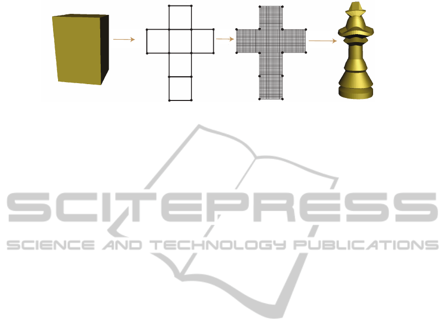
Flattening

Editting

Figure 1: The initial cube’s connectivity map and its subdivided version.The cube’s vertices are manipulated and a chess piece

is obtained. The connectivity map’s indices are shown beside them. (a, b)

indicates the vertex with index (a, b) at resolution

every vertex of the polyhedron based on its Cartesian

coordinates. These integer indices refer to entries of

a 2D array storing vertices’ 3D positions. Using such

connectivity maps, simple operations in 2D are de-

ﬁned to ﬁnd the neighbors of a face or vertex. Indeed,

simplicity of the proposed connectivity maps result

simple operations for connectivity inquiries. Using

such connectivity maps, all the vertices, edges and

face’s connectivities can be found using algebraic re-

lationships. In summary, our approach is devoted to

deﬁning the connectivity and the topology of geomet-

ric models as a primary goal while the geometry and

its modiﬁcations (including subdivision schemes) are

added as a secondary goal.

Although we use simple polyhedrons, complex

objects can be created using this data structure. For

creating complex shapes, the initial simple polyhe-

dron can be subdivided using various subdivision

schemes such as linear, Catmull-Clark or Loop sub-

division. The location of subdivided vertices can then

be modiﬁed (manually or automatically) using defor-

mation techniques or remeshing methods to create the

desired shapes and holes and sharp features can also

be added. Note that in this representation, it is only

necessary to store vertex positions since the connec-

tivity of edges and faces is implicit (See Fig 1).

Our main contribution is to introduce connectivity

maps for polyhedrons. The coordinates of the con-

nectivity maps’ vertices are considered as indices that

can address adjacency queries and provide 3D loca-

tions. Initial connectivity maps are provided and com-

plicated pre-processing steps are not required. After

establishing the initial connectivity maps, subsequent

resolutions are formed based on the initial connec-

tivity maps. Using the proposed connectivity maps

and the indexing method, adjacency and hierarchical

queries are addressed using fast and straightforward

algebraic relationships.

The rest of the paper is organized as follows: Re-

lated work is discussed in Section 2. We discuss the

indexing scheme in Section 3. Hierarchical traversal

and neighborhood vectors are discussed in Section 4.

We clarify how to apply Loop and Catmull-Clark sub-

division using our method in Section 5. Hierarchical

mesh editing is discussed in Section 6. We describe

some possible methods to generate complex objects

with simple connectivities in Section 7. Extracting

connectivity information of geometry images is de-

scribed in Section 8 and ﬁnally we compare the speed

of the proposed indexing with that of the half-edge in

Section 9.

2 RELATED WORK

Generating an object using subdivision schemes such

as Loop and Catmull-Clark is a standard method for

geometric modeling (Loop, 1987; Catmull and Clark,

1998). The half-edge and quadtree are two commonly

used data structures to support subdivision schemes

(Weiler, 1985; Kettner, 1998; Samet, 2005; Zorin

et al., 1997). However, when the information stored

by a data structure becomes very large, it is inefﬁcient

to use pointer based data structures for storing con-

nectivity information (Samet, 1990; Samet, 1985). In

order to avoid pointers, some indexing methods have

been proposed to index mesh vertices and faces.

Proposed indexing methods for quadtrees (Samet,

1985; Gargantini, 1982) can be used for represent-

ing meshes. However, as a very important inquiry

for mesh processing, neighborhood ﬁnding is not efﬁ-

cient enough for interactive applications. In our work,

we derive some simple algebraic operations for ﬁnd-

ing neighbors of a given face or vertex. The beneﬁt

of algebraic operations is not only that neighbors of a

face or vertex can be found in constant time, but fur-

ther faces or vertices such as neighbors of neighbors

(more than 1-ring neighborhood) are also accessible

in constant time.

Patch-based methods generally divide the mesh

CONNECTIVITY MAPS FOR SUBDIVISION SURFACES

(0,0)0 (1,0)0

(2,0)0

(2,1)0

(1,1)0(0,1)0

(0,2)1

(0,0)1

(0,1)1

(2,2)1

(2,0)1

(4,0)1

(4,2)1

(1,0)0

(2,0)0

(1,1)0

(1,2)0

(1,3)0

(1,4)0

(0,3)0

(0,2)0

(2,1)0

(2,2)0

(2,3)0

(2,4)0

(3,2)0

(3,3)0

(2,0)1 (4,0)1

(2,2)1

(0,4)1

(0,5)1

(0,6)1

(2,8)1

(3,8)1

(4,8)1

(6,6)1

(6,4)1

(6,5)1

(4,2)1

(0,0)0

(1,0)0

(2,0)0

(0,1)0

(0,2)0

(1,2)0

(2,1)0

(2,2)0

(0,0)1

(2,0)1

(4,0)1

(0,2)1

(0,4)1

(2,4)1 (4,4)1

(4,2)1

(4,1)1

(0,0)0

(3,0)0

(0,4)0

(3,4)0

(0,2)0 (0,4)1

(0,0)1

(6,0)1

(0,8)1

(6,8)1

(6,4)1

(3,2)0

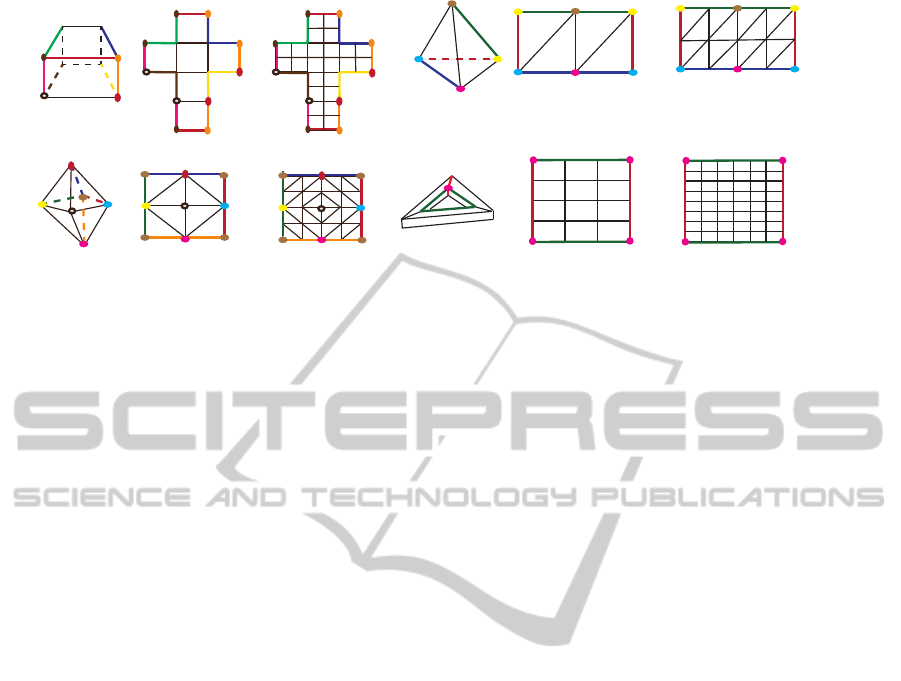
Figure 2: A cube, tetrahedron, octahedron and a toroidal polyhedron and their 2D domain at the ﬁrst and the second resolu-

tions. (a, b)

indicates the index of a vertex at resolution r. Vertices or edges with the same colors on 2D domain are copies of

one vertex or edge in 3D. Boundary edges are highlighted by thicker lines.

into collection of separated faces and consider arrays

for each single patch (Bunnell, 2005; Shiue et al.,

2005; Peters, 2000). These methods are speciﬁcally

designed for handling subdivision schemes specially

Catmull-Clark subdivision. Using the method pre-

sented by (Bunnell, 2005), the surface can be divided

into some patches connected by an edge based data

structure such as the half-edge and ﬁne resolution ver-

tices are stored in separate 2D arrays. This method

is designed for general quad meshes resulting from

Catmull-Clark subdivision but it cannot support tri-

angular meshes and Loop subdivision. In compari-

son with (Bunnell, 2005), we propose an indexing for

important simple shapes. We can support Loop and

Catmull-Clark subdivision schemes and we establish

algebraic relationships for neighbors of boundary ver-

tices that enable us to avoid half-edge data structure

at the ﬁrst resolution. Although we use simple poly-

hedrons for establishing connectivities, our method is

not restricted to simple objects. Using remeshing and

sketch-based deformation techniques and supporting

sharp features and holes, we can create complex ob-

jects that beneﬁt from polyhedron’s simplicity.

Shiue et al. use an alternative way to apply sub-

division methods (Shiue et al., 2005). They initially

subdivide the mesh using an edge based data structure

in a pre-processing step. They then divide the mesh

into some patches with repetitive boundary vertices.

Each patch’s vertices is indexed using a spiral index-

ing and located in a 1D array. Using a spiral index-

ing methods, close vertices may get unrelated indices.

Therefore, this method does not establish a straight-

forward relationship for neighborhood ﬁnding and ac-

cess to neighbors of a vertex needs to traverse the spi-

ral. Consequently, previous patch based reﬁnement

methods are speciﬁcally designed to support subdi-

vision methods and they do not consider the shape’s

connectivity relationship which is an important aspect

of the geometric modeling.

Since our method uses a ﬂattened regular shape

for meshes, it is also somehow related to the

parametrization problem (Hormann et al., 2007). Pa-

rameterization is used for different applications such

as texture mapping, mesh editing and Geometry Im-

ages. For creating Geometry Images, Gu et al. (Gu

et al., 2002) uses cuts in order to ﬂatten a general

topology object. They then resample the ﬂattened ob-

ject to create a regular surface called a ”geometry im-

age”. They generate an image to store the vertex loca-

tions of objects in such a way that red, green and blue

components of an image represent x,y and z locations

of a vertex respectively. Boundary extension rules are

not straightforward in this method; therefore, connec-

tivity relationships are hard to ﬁnd for boundaries.

Praun and Hoppe (Praun and Hoppe, 2003) pro-

pose a spherical parameterization to generate regu-

lar meshes of genus 0 objects using the octahedron,

cube or tetrahedron. They parameterize an object to

a sphere then use one of the mentioned polyhedra

for resampling and create a regular mesh. Meshes

obtained from (Praun and Hoppe, 2003) are depen-

dent on the geometry of initial shapes that have to

be remeshed. Therefore, small changes in geome-

try images need modiﬁcation of the initial shape, re-

quiring an expensive reparameterization of the entire

mesh. However, our method begins with a 2D regu-

lar domain (connectivity map) for an efﬁcient access

to the connectivity information, and also maintains

this regularity during geometry changes (editing, de-

formation, and subdivision operations). Additionally,

changing the mesh at any resolution can be propa-

gated to further resolutions without using expensive

operations. Because of this, our method can be a good

complementary work for Geometry Images. In sum-

mary, to have a comparable title with (Gu et al., 2002),

our work can be conceptually considered as Connec-

tivity Images.

GRAPP 2012 - International Conference on Computer Graphics Theory and Applications

3 THE INDEXING SCHEME

Since the indexing method works based on 2D vectors

of Cartesian coordinates, the initial polyhedron must

be ﬂattened. There are many ways to unfold these ini-

tial objects but we use the one in which connectivity

maps have easier boundary rules (see Figures 1 and

2). We then locate every vertex of the polyhedron on

integer Cartesian coordinates. These integer coordi-

nates are used as the vertices’ index. Working with

this simple shape is not enough for many applications

and it only creates a base topology of shapes, there-

fore it is necessary to support subdivision. To keep

track of the levels of subdivision, we also use an extra

index, the subscript index, as the resolution or level of

subdivision. Therefore, a vertex with index (a, b)

a and b steps far from the origin in X and Y directions

at resolution r.

(a,b)

[a,b]

(a+1,b)

(a+1,b+1)

(a,b+1)

(a)

(a,b+1)

(a,b)

(a+1,b)

(a+1,b+1)

(a,b)

(a+1,b)

(a+1,b+1)

(c)(b)

Figure 3: (a) A quadrilateral face, and the index of its faces

and vertices. (b,c) Two forms of triangular faces of a quadri-

lateral face.

We use the resulting 2D integer coordinates as in-

dices to a 2D array containing the locations of ver-

tices. We also use the same index for addressing

faces. The index of the left-bottom vertex of a face is

considered as its index. Therefore, based on a face’s

index, indices of its vertices are computable and vice

versa. Indeed, if the left bottom vertex of a face is

(a, b)

, vertices making this face have indices (a, b)

(a + 1, b)

, (a + 1, b + 1)

and (a, b + 1)

. This rela-

tionship is valid for quadrilateral faces. Because of

the regularity of triangular faces in our initial poly-

hedron, it is possible to assign faces’ indices to quads

formed by triangles. There are two possible triangular

faces for each quad (see Fig 3). All triangular faces

of a tetrahedron has the form of Fig 3.b. However,

based on the region in which a quad falls (see Fig 2),

triangles of an octahedron can have forms of Fig 3.b

or Fig 3.c.

4 HIERARCHICAL TRAVERSAL

AND NEIGHBORHOOD

VECTORS

Hierarchical Traversal. In our method, when a face is

subdivided using linear, Catmull-Clark or Loop sub-

division methods, it is split into four faces after each

level. Fine faces generated by splitting a coarse face

are called children and the coarse face is called par-

ent. One of the important hierarchical operations is to

ﬁnd indices of all the children of a given face [a, b]

(we use [a, b]

for faces’ indices to distinguish them

from vertices’ indices represented by (a, b)

) at reso-

lution r + k

or ﬁnding the index of its parent at reso-

lution r − k

, k

> 0).

To maintain efﬁcient hierarchical operations and

regularity, after each level of subdivision, we use

the same 2D coordinates for the vertices from pre-

vious levels. Since every face is split into four faces,

the length of unit vectors is divided by two. There-

fore, unit vectors (0, 1)

and (1, 0)

are equal to

2 × (0, 1)

r+1

and 2 × (1, 0)

r+1

respectively. Result-

ing from these relationships, we can derive the hierar-

chical relationship of a vertex at different resolutions.

Equations 1 and 2 imply correspondent indices of ver-

tex (a, b)

at resolutions r + k and r − k respectively.

Note Equation 2 must only applied to vertex-vertices.

(a, b)

= (2

a, 2

r+k

(1)

(a, b)

= (

)

r−k

(2)

Similarly, a face with index [a, b]

has children

with indices [2a, 2b]

r+1

, [2a + 1,2b]

r+1

, [2a, 2b +

r+1

and [2a + 1, 2b + 1]

r+1

(Fig 5). In general af-

ter n (n > 0) levels of subdivision, a face with index

[a, b]

would have children with indices [c, d]

r+n

which 2

a ≤ c < 2

n+1

a and 2

b ≤ d < 2

n+1

b. There-

fore, a face with index [a, b]

has a parent with index

[









]

r−n

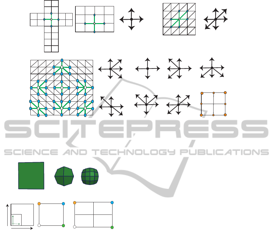
Neighborhood Vectors. Since each vertex of the

connectivity map is located on an integer 2D Carte-

sian coordinate, there are vectors that connect vertex

v to all its neighbors. These vectors are called neigh-

borhood vectors which differ based on the underlying

polyhedra’s connectivity maps. Figure 4 illustrates

them for the initial polyhedra.

Neighborhood vectors illustrated in Figure 4 are

used for internal vertices. Unfolded polyhedrons have

boundary edges and vertices which are shown in Fig-

ure 2. Since boundary vertices have multiple copies in

connectivity maps, their neighbors are split into mul-

tiple locations surrounding each copy. As a result,

to determine neighbors of boundary vertices, their

copies must also be found (Fig 2).

CONNECTIVITY MAPS FOR SUBDIVISION SURFACES

(0,1)

(1,0)

(0,-1)

(-1,0)

(0,1)

(1,1)

(1,0)

(0,-1)

(-1,-1)

(-1,0)

(a)

(b)

(0,1)

4 5

(c)

(1,1)

(1,0)

(1,-1)

(0,-1)

(-1,0)

(0,1)

(1,0)

(0,-1)

(-1,-1)

(-1,0)

(-1,1)

(0,1)

(1,0)

(0,-1)

(0,1)

(1,0)

(1,-1)

(0,-1)

(-1,-1)

(-1,0)

(0,1)

(1,1)

(1,0)

(0,-1)

(-1,-1)

(-1,0)

(1,1)

(0,1)

(-1,1)

(1,0)

(0,-1)

(-1,0)

(0,2

r+1

)

r+1

)

r+1

,0)

(0,0)

(-1,1)

(0,1)

(1,0)

(-1,0)

(0,-1)

(1,-1)

Figure 4: (a) Neighborhood vectors for a cube or a toroidal polyhedron . (b) Neighborhood vectors for a tetrahedron. (c)

Seven possible neighborhood vectors for an octahedron. Based on the region in which the vertex falls, neighborhood vectors

can be determined. For example, if a vertex falls in the region 0 < a, b < 2

, its neighborhood vector is of the condition 1.

(a)

(b)

(c)

(0,1)

r+1

(a,b)

[a,b]

(d) (e)

(f)

(1,1)

(1,0)

r+1

(a+1,b)

(a+1,b+1)

(a,b+1)

(2a,2b+2)

r+1

(2a+2,2b+2)

r+1

(2a,2b)

r+1

(2a+2,2b)

r+1

[2a+1,2b]

r+1

[2a+1,2b+1]

r+1

[2a,2b]

r+1

[2a,2b+1]

r+1

Figure 5: (a) A face at resolution 0. (b) The patch obtained

from (a) at resolution 1. (c) The patch obtained from (a)

at resolution 2. (d) Unit vectors at resolutions r and r + 1.

(e) A face’s index and its vertices’s indices at resolution r.

The patch obtained from (e) and it’s faces’ indices. Green

indices are vertex indices and black ones are face’s indices.

To recognize if A = (a, b)

is a boundary vertex,

we check whether it falls along one of the bound-

ary edges of the initial connectivity map. Consider

boundary edge e connecting two ﬁrst resolution ver-

tices P = (x

, y

)

and Q = (x

, y

)

. A is located

on boundary edge e if its index (a, b)

is in be-

tween of the indices of P and Q at resolution r. Us-

ing Equation 1, P and Q respectively have indices

, 2

)

and (2

, 2

)

at resolution r. There-

fore, A = (a, b)

is located on e if min



, 2



≤

a ≤ max



, 2



and min



, 2



≤ b ≤

max



, 2



. This relationship is general for all

boundary edges. However, boundary edges of the pro-

posed polyhedrons typically have simpler conditions.

For instance, the toroidal polyhedron has four bound-

ary edges and A = (a,b)

is located along one of the

boundary edges when a = 0, b = 0, a = 3 × 2

b = 4 × 2

(Fig 2).

After recognizing that a vertex is located on the

connectivity map’s boundary, its neighbors have to be

determined. As we discussed earlier, to ﬁnd neigh-

bors of a boundary vertex, its copies are required.

Copies of vertices at the initial resolution are known

based on the connectivity map. To determine copies

of a boundary vertex at resolution r, we propose a

general method that can be applied to all the proposed

polyhedrons. This general method’s basic idea is to

ﬁrst ﬁnd edge e on which boundary vertex A is lo-

cated (Fig 6). Afterwards, having the e’s copy which

is obtainable from the connectivity map, the index of

A’s copy is determined. We describe the mathemati-

cal representation of this issue in the following.

Let A = (a, b)

be a boundary vertex whose copy,

C = (c, d)

, is required (see Fig 6). A is located

on a ﬁrst resolution edge e connecting P = (x

, y

)

and Q = (x

, y

)

. P and Q respectively have copies

Z = (x

, y

)

and W = (x

, y

)

at the ﬁrst resolution.

A can be written as a linear combination of P and Q.

A = (1 − α)P + αQ. Using copies of P and Q, the

copy of A can be determined as C = (1 − α)Z + αW .

For instance, consider the vertex with index A =

(a, b)

= (0, 21)

on the cube’s 2D domain (Fig 6).

Since a = 0, this vertex is located on the edge con-

GRAPP 2012 - International Conference on Computer Graphics Theory and Applications

P=(xp,yp)

Q=(xq,yq)

W=(xw,yw)

Z=(xz,yz)

P=(0,2)

Q=(0,3)

A=(0,21)

C=(8,3)

C=(c,d)

W=(1,0)

Z=(1,0)

A=(a,b)

Figure 6: Left: copy of A = (a, b)

is shown by a white vertex. Copy of A, C = (c, d)

, is found using the described general

method. e and its copies are respectively highlighted by green and orange vectors. Right: an example of the general method

to ﬁnd the copy of (0, 21)

necting vertices with indices P = (0, 2)

= (0, 16)

and Q = (0, 3)

= (0, 24)

. Therefore, (0, 21)

= (1−

α)(0, 16)

+ α(0, 24)

⇒ α =

. Since copies of P

and Q have respectively indices Z = (1, 1)

= (8, 8)

and W = (1, 0)

= (8, 0)

. C =

(8, 8) +

(8, 0)

(8, 3)

After ﬁnding copies of a boundary vertex (A),

neighborhood vectors are applied on A and its copies.

Resulting neighbor vertices are stored in set N. Af-

terwards, Repetitive Vertices of N and those vertices

that fall out of the 2D domain are excluded. To dis-

card repetitive vertices, we keep neighbors that are di-

rectly obtained by applying neighborhood vectors on

A and then eliminate their copies. It is not necessary

to do the same process for every single resolution. It

is enough to ﬁnd neighbors of boundary edges at one

resolution and then extend it to next resolutions using

Equation 1.

5 SUBDIVISION METHODS

To generate complex objects, it is possible to subdi-

vide the initial object, manipulate resulting vertices

in a small number of iterations until the desired ob-

ject is formed. After an application of linear, Loop or

Catmull-Clark subdivision, each face is split into four

faces, and some new vertices are generated. To sup-

port the possibility of creating more advanced shapes

and also to demonstrate the usefulness of the indexing

method proposed for the connectivity maps, in this

section, we describe how to perform smooth subdivi-

sion schemes using the indexing method.

5.1 Catmull-Clark Subdivision

Each iteration of Catmull-Clark subdivision requires

a face split operation and also a relocation of resulting

vertices through subdivision masks. We have already

described hierarchical relationships resulting from the

face split in Section 4. Here we discuss how to apply

subdivision masks on the quad faces of the cube and

toroidal polyhedron. Masks of Catmull-Clark subdi-

vision are as follows (Halstead et al., 1993):

i+1

∑

(3)

i+1

+ e

+ f

i+1

j−1

+ f

i+1

(4)

i+1

n − 2

∑

i+1

(5)

In the neighborhood of vertex v

, f

i+1

, f

i+1

,...,

i+1

and e

i+1

, e

i+1

, ..., e

i+1

are respectively face-

vertices and edge-vertices and v

i+1

is the vertex-

vertex at the resolution i + 1.

After one level of subdivision, a face with index

[a, b]

is split into four faces [2a, 2b]

r+1

, [2a +1, b]

r+1

[2a + 1, 2b + 1]

r+1

and [2a, 2b + 1]

r+1

as illustrated

in Fig 7. These faces’ vertices must be computed

using Catmull-Clark subdivision masks. Applying

Equation 3 on face [a, b]

, the face-vertex Q

(1,1)

(2a + 1, 2b + 1)

r+1

is computed using the following

equation:

(1,1)

(0,0)

+ P

(1,0)

+ P

(1,1)

+ P

(0,1)

, (6)

CONNECTIVITY MAPS FOR SUBDIVISION SURFACES

where P

(0,0)

, P

(1,0)

, P

(1,1)

, and P

(0,1)

respectively have

indices (a, b)

, (a + 1, b)

, (a + 1, b + 1)

, and (a, b +

After ﬁnding face vertices, edge-vertices (2a +

1, 2b)

r+1

, (2a + 2, 2b + 1)

r+1

, (2a + 1, 2b + 2)

r+1

and

(2a, 2b + 1)

r+1

are computed using (4). For exam-

ple, as demonstrated in Fig 7 (d), the edge-vertex

(1,2)

= (2a + 1, 2b + 2)

r+1

is determined by:

(1,2)

(1,1)

+ Q

(1,3)

+ P

(0,1)

+ P

(1,1)

, (7)

where Q

(1,1)

, Q

(1,3)

, P

(0,1)

, and P

(1,1)

respectively

have indices (2a + 1, 2b + 1)

r+1

, (2a + 1, 2b + 3)

r+1

(a, b + 1)

, and (a + 1, b + 1)

After ﬁnding all edge-vertices, it is possible to

compute the vertex-vertices. Vertex-vertices are in

fact existing vertices at the coarser resolution trans-

lated to new positions. When (a, b)

is a regular ver-

tex, the involving neighboring vertices in the vertex-

vertex mask can be easily found. As demonstrated in

Fig 7 (e), we need face vertices with indices (2a +

1, 2b + 1)

r+1

, (2a − 1, 2b + 1)

r+1

, (2a − 1, 2b − 1)

r+1

and (2a + 1, 2b − 1)

r+1

, and edge vertices with in-

dices (a −1, b)

, (a+1, b)

, (a, b+1)

and (a, b −1)

Using these indices and Equation 5 the position of

(2a, 2b)

r+1

can be computed.

Subdivision

[a,b]

(2a,2b)

r+1

(2a+2,2b)

r+1

(2a,2b+2)

r+1

(2a+2,2b+2)

r+1

(a,b+1)

(a+1,b+1)

(a+1,b)

(a,b)

(2a+1,2b+1)

r+1

(2a+1,2b+2)

r+1

(2a+1,2b+1)

r+1

(a,b+1)

(a+1,b+1)

(2a+1,2b+3)

r+1

(2a,2b)r+1

(a,b+1)

(a-1,b)

(a,b-1)

(2a-1,2b-1)r+1

(2a+1,2b-1)

r+1

(a+1,b)

(2a-1,2b+1)

r+1

(2a+1,2b+1)

r+1

(b)

(a,b+1)

(a,b)

(a+1,b)

(a+1,b+1)

[2a,2b]

r+1

(a)

(c)

(d)

(e)

Figure 7: (a) Face [a, b]

and its vertices. (b) Children of

face [a, b]

at resolution r + 1 and their vertices. ((c), (d),

(e)) Black vertices are vertices at resolution r. Orange, blue

and red vertices represent face, edge and vertex-vertices re-

spectively.

It is also necessary to handle extraordinary ver-

tices (n 6= 4). Since each step of Catmull-Clark subdi-

vision does not introduce any new extraordinary ver-

tex the set of extraordinary vertices resulting from

this subdivision correspond to the extraordinary ver-

tices of the initial connectivity map. Therefore, the

index of this kind of vertices is predictable during

subdivision. In fact, using Equation 1, given the

index of the extraordinary vertices at the ﬁrst res-

olution, the index of extraordinary vertices at any

resolution r can be found. For example, extraor-

dinary vertices of the cube are: (2

, 0)

, (2

r+1

, 0)

r+1

, 2

r+1

)

, (2

r+1

, 2

)

, (0, 2

r+1

)

, (2

, 2

r+1

)

, (3 ×

, 2

r+1

)

, (0, 3 × 2

)

, (2

, 3 × 2

)

, (2

r+1

, 3 × 2

)

(3 × 2

, 3 × 2

)

, (2

, 2

r+2

)

and (2

r+1

, 2

r+2

)

. So by

keeping track of extraordinary vertices and applying

appropriate masks to them, we can subdivide the ini-

tial polyhedra. We applied Catmull-Clark subdivision

to the cube and toroidal polyhedron. Figure 8 shows

a toroidal polyhedron at three different resolutions.

Figure 8: The toroidal polyhedron at three different

Catmull-Clark subdivision levels.

5.2 Loop Subdivision

Another common subdivision method is Loop’s

scheme (Loop, 1987). In this triangular-based

scheme, each triangular face is split to four triangles.

There are two types of masks for Loop subdivision:

edge-vertex and vertex-vertex masks. Using the nota-

tion demonstrated in Fig. 9, these masks are deﬁned:

i+1

(8)

i+1

= (1 − nα)v

+ α

∑

(9)

α =

(

− (

cos

(2π)

)

) (10)

We discuss the case of neighborhood vectors for a

tetrahedron. The octahedron case is similar (note that

it is also possible to apply Loop subdivision on the

toroidal polyhedron and cube by splitting every quad

to two triangles). To apply the mask of edge-vertices

presented in Equation 8, vectors (1, 0)

, (1, 1)

and

(0, −1)

are needed. For vertex-vertices however, all

the neighborhood vectors presented in Section 4 (also

Fig 4) for the tetrahedron are required to ﬁnd neces-

sary neighbors. Extraordinary vertices are handled

similar to Catmull-Clark. Figure 10 illustrates the

result of Loop subdivision on the initial tetrahedron.

5.3 Holes and Sharp Features

There are many objects that have sharp features and

holes. A data structure should be able to support these

GRAPP 2012 - International Conference on Computer Graphics Theory and Applications

i+1

Figure 9: Left: necessary neighborhood vectors for comput-

ing edge vertices. Right: necessary neighborhood vectors

for computing vertex vertices.

Figure 10: Two left ﬁgures are the tetrahedron at the second

and third resolutions. Three right ﬁgures are the cube with

sharp edges along the bottom over three successive levels of

subdivision. The last subdivided cube is depicted in another

view.

features to make realistic and useful objects. In this

section, we describe how to handle holes and sharp

features.

5.3.1 Holes

To support objects with holes, individual faces at any

arbitrary resolution are tagged as empty. As discussed

in Section 4, it is possible to ﬁnd all the faces in the

resolution r + k that are children of a face at the reso-

lution r. Using this property, all children of an empty

face and its related vertices are marked as empty in

further resolutions. Once we render the mesh, empty

faces and their vertices (except the vertices of the

boundary) are ignored. A cubic B-spline subdivi-

sion mask can be applied to the edges (vertices of the

boundary) of these holes. Figure 11 shows a cube

with three holes at three successive levels of subdivi-

sion.

5.3.2 Sharp Features

To support sharp features, we use the method de-

scribed in (DeRose et al., 1998) and (Hoppe et al.,

1994) for Catmull-Clark and Loop schemes respec-

tively. In general, for objects that have sharp features,

there are three kinds of vertices. Normal vertices, ver-

tices with no sharp edges; creases, vertices with two

sharp edges that a cubic B-Spline mask should be ap-

plied to them; and corners, vertices with more than

two sharp edges whose positions are changed.

Consider a sharp edge between (a, b)

and (a +

1, b)

, after k levels of subdivision all the edges be-

tween a pair of vertices in the range (2

a, 2

r+k

and

a + 2

, 2

r+k

are sharp. Therefore, vertices of

(10,22)

(10,20)

(14,20)

(14,22)

(5,11)

(5,10)

(7,10)

(7,11)

(20,44)

(20,40)

(28,40)

(28,44)

Figure 11: Top: A cube is subdivided using linear subdivi-

sion twice, three holes are made in the cube and it is subdi-

vided twice using Catmull-Clark subdivision. Bottom: The

connectivity maps of the top ﬁgures. It is possible to keep

the track of empty faces’ indices during the subdivision that

are highlighted by white blocks.

Figure 12: The evolution of a cat from a cube using direct

manipulations of vertices.

these edges are known during resolutions and a sharp

or corner mask is applied to them. Figure 10 shows

a cube with sharp edges along the bottom over three

successive levels of subdivision.

It is not necessary to tag all the sharp edges at fur-

ther resolutions. To apply different masks to sharp

features, we keep an array including all sharp features

at the coarsest resolution ((a, b)

). We ﬁrst subdi-

vide the mesh without considering sharp tags and then

ﬁnd all the sharp edges’ vertices at current resolution

(from (2

a, 2

r+k

to (2

a + 2

, 2

r+k

) and modify

their positions by the appropriate mask.

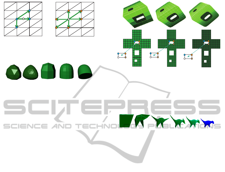
6 HIERARCHICAL MESH

EDITING

To generate a mesh, one can modify an initial polyhe-

dron, subdivide and modify, and add features to it un-

til the desired shape is achieved (Fig 12 and 13). Dur-

ing this process, one may want to go back to coarser

resolutions and makes some modiﬁcations. To mod-

ify the model at a coarser resolution, we can use

the connectivity map of the coarse resolution, mod-

ify some vertices and propagate the modiﬁcation to

the current resolution using some local subdivision

masks.

Consider vertex v is modiﬁed by vector ∆v. ∆v has

CONNECTIVITY MAPS FOR SUBDIVISION SURFACES

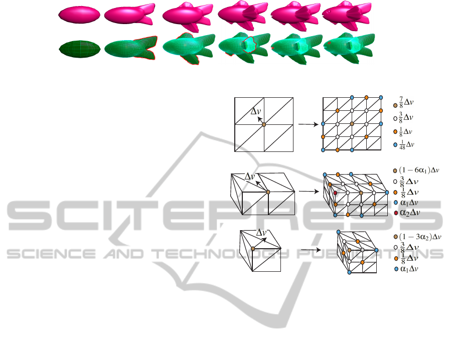
Figure 13: The evolution of a ﬁsh from a subdivided cube using sketches.

local contributions at subsequent resolutions. Instead

of subdividing the entire mesh, we can determine

the contributions and modify affected vertices. Since

there are extra-ordinary vertices in the proposed poly-

hedrons, there are three types of local masks based on

the location of the modiﬁed vertex. These three cases

are: 1. a regular vertex without any direct connection

to an extraordinary vertex; 2. a regular vertex adjacent

to an extra-ordinary vertex; 3. an extra-ordinary ver-

tex. Figure 14 illustrates these possible cases for the

toroidal polyhedron. In Figure 14, the extra-ordinary

vertex has valence 3 and its subdivided vertex is high-

lighted by a red vertex when it is located in a regular

vertex’s neighborhood. Therefore, setting n to 6 and 3

in Equation 10 respectively results α

and α

shown

in Figure 14 . These possible cases can also be de-

termined using a similar method for other proposed

polyhedrons and Catmull-Clark subdivision.

Note for case 2, the extra-ordinary vertex may be

located at a different edge as shown in Fig 14. In this

situation, the local mask is rotated in such a way that

extra-ordinary vertex of the mask is matched with the

extra-ordinary vertex of the regular vertex’s neighbor-

hood.

We do not consider the case of two extra-ordinary

vertices in one neighborhood which occurs only at the

ﬁrst resolution. For low resolution objects, it is efﬁ-

cient to globally subdivide the 2D domain consider-

ing ∆v for the modiﬁed vertex and 0 for other ver-

tices. However, vertex modiﬁcations at high resolu-

tions using global subdivision need huge amount of

calculations therefore it is more efﬁcient to apply the

local subdivision for the modiﬁcation and recursively

propagate it to subsequent resolutions.

7 OTHER GEOMETRIC

MANIPULATIONS

So far, we have shown that our method can efﬁciently

support subdivision schemes. In general, any solitary

geometric operation on the initial connectivity map is

very simple and efﬁcient. However, any major geo-

metric change may require a new distribution of ver-

tices in a multi scale manner. To show that the pro-

posed method can be employed in various scenarios,

Figure 14: Local subdivision masks foe described case.

Top: Case 1. Middle: Case 2. Bottom: Case 3. Right

ﬁgures represent the modiﬁed vertices’ locations after one

level of subdivision due to the modiﬁcation of ∆v. The mod-

iﬁcation values of the colorful ovals are presented at the

right of each ﬁgure. Vertices highlighted by colorful ovals

get the same modiﬁcation values as appeared near the ovals.

we use sketch-based deformation and remeshing tech-

niques to generate more complex objects.

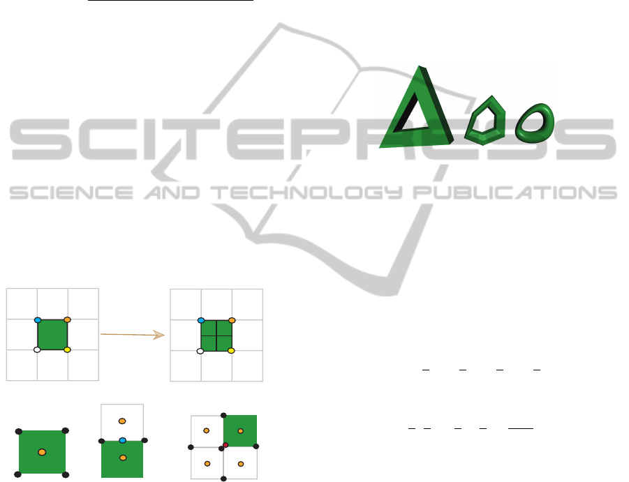
7.1 Sketch-based Deformation

To deform a model, the positions of vertices are some-

how modiﬁed. Such modiﬁcations can be done sim-

ply using direct manipulation of vertices at any reso-

lution (see Fig 1 and 12) or using some deformation

methods. To show the capacities of our method, we

have employed the deformation technique proposed

in (Pusch and Samavati, 2010) in a sketch-based mod-

eling interface to deform an initial shape to make

more complex shapes as the one demonstrated in Fig

13.

Another beneﬁt of our method for the sketch-

based modeling is to provide a very regular meshing

of closed, sketched curves. There are several appli-

cations in the sketch-based modeling in which a user

draws a closed curve and a 3D mesh is obtained from

the curve (Olsen et al., 2009; Nealen et al., 2007). It

is appropriate that the resulting mesh of these appli-

GRAPP 2012 - International Conference on Computer Graphics Theory and Applications

cations becomes regular with very low number of ex-

traordinary vertices (Nealen et al., 2009; Nasri et al.,

2009). To achieve this goal, we start with an octahe-

dron and ﬁt its base to the sketched curve by snap-

ping vertices of the octahedron’s base to the sketched

curve (Olsen et al., 2009). The base of an octahe-

dron is a square at the ﬁrst resolution. After each

level of subdivision, the base of the octahedron be-

comes smoother and can approximate the curve in a

better way. By repeating the subdividing and ﬁtting

process, we can increase the accuracy of the stroke’s

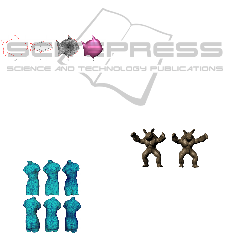
approximation as demonstrated in Fig 15. For inﬂa-

tion, we can use methods described in (Olsen et al.,

2009; Igarashi et al., 2007). The resulting mesh is

very regular and only has six extraordinary vertices.

Figure 15: (a) A sketched curve. (b) The base of the octa-

hedron is ﬁt to the curve. (c) The mesh resulted from sub-

dividing and ﬁtting process described above. (d) Mesh is

rendered using smooth shading.

7.2 Remeshing Techniques

Remeshing methods typically try to approximate a

target mesh using a simple base mesh such as a subdi-

vided polyhedron. One possible way to approximate

a general mesh is to use a method similar to (Sharf

et al., 2006). In (Sharf et al., 2006), the target mesh

is approximated using a simple base mesh (sphere).

The base mesh’s vertices are moved in the direction

of their normals (evolving process) until the distance

Figure 16: Left ﬁgures are the venus with a general mesh.

Middle and right ﬁgures are the approximation of left ﬁg-

ures using a method similar to (Sharf et al., 2006) at two

successive levels of approximation.

between the vertices of the base mesh and the target

mesh is less than a threshold. After the evolving pro-

cess, the base mesh is locally subdivided to have a

better approximation of the target. The base mesh

again evolves and this process continues until the de-

formable model is close enough to the target mesh.

We use a similar approach but we subdivide the whole

base mesh to approximate the target mesh. Figure 16

illustrates this approach to approximate the Venus.

8 GEOMETRY IMAGES

Our connectivity map can also be used as a comple-

mentary tool for deforming, modifying and subdivid-

ing meshes resulting from geometry images (Losasso

et al., 2003; Praun and Hoppe, 2003). To apply our

proposed method on a geometry image resulting from

the spherical parameterization method, we must ﬁrst

synchronize the resolutions. This means that num-

ber of vertices in the geometry image and the num-

ber of vertices of the connectivity map must be equal.

Therefore, we subdivide the initial polyhedron (con-

sistent with one that is used by the spherical parame-

terization) until we get the same resolution. Then we

use the geometry image’s data to set the vertex posi-

tions of our indices. We now are able to edit, modify

and subdivide the mesh. Figure 17 illustrates an ob-

ject obtained by geometry image’s approach before

and after applying Loop subdivision.

Figure 17: Left: an object obtained from geometry images.

Right: left ﬁgure after one level of loop subdivision.

9 SPEED EFFICIENCY

One of the most common data structures for meshes is

the half-edge (Weiler, 1985; Kettner, 1998). This data

structure needs to save edges, pairs of edges, vertices

(their location and their connection to half-edges) and

faces. In our method, the only information that must

be stored is the location of vertices and the initial con-

nectivity map’s indices. Connectivity information is

efﬁciently extracted from these indices.

CONNECTIVITY MAPS FOR SUBDIVISION SURFACES

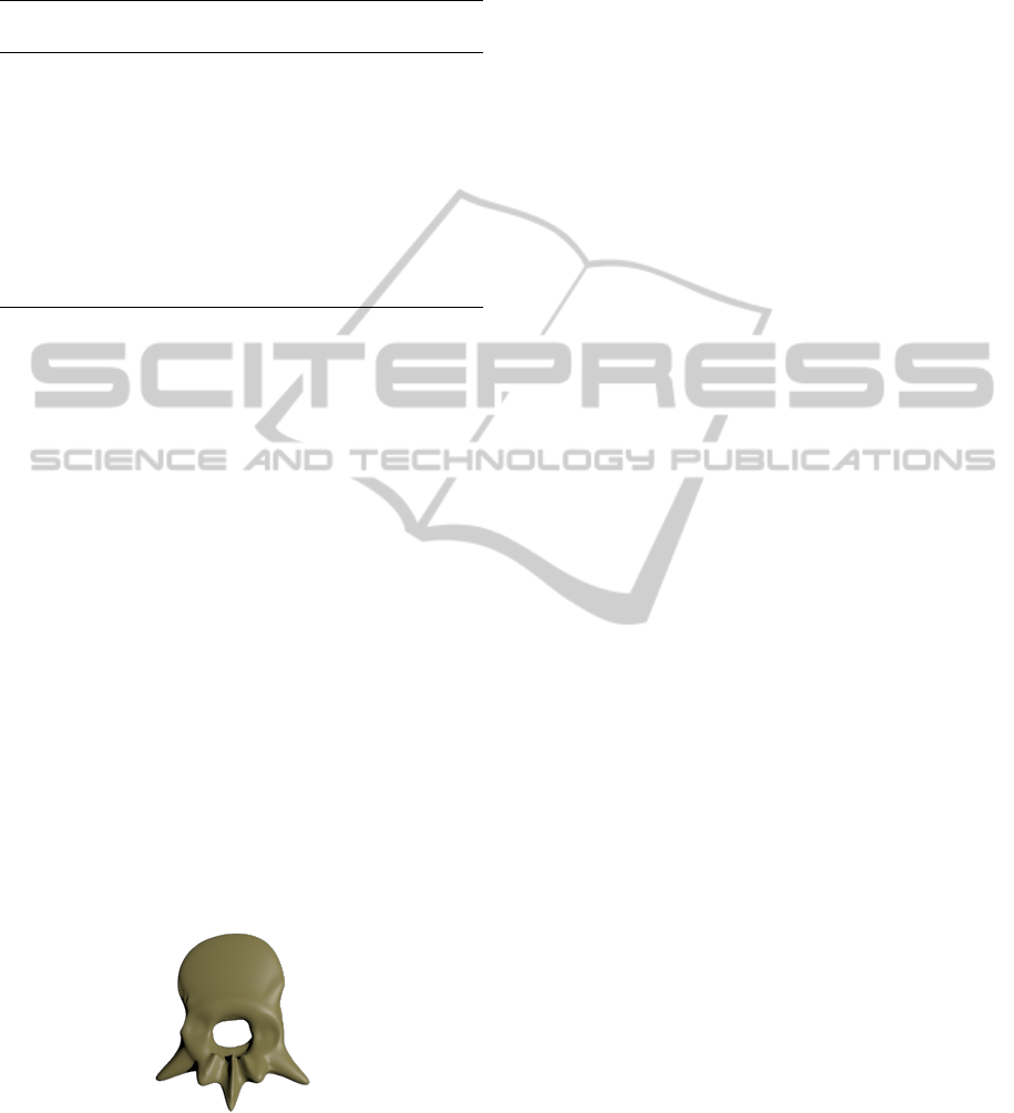
Table 1: Number of faces in every step of Loop subdivision

of the tetrahedron and run-time of our method (connectiv-

ity map) and the half-edge. NA shows an extremely large

number.

Steps of No. of Our method Half-edge

Subdivision faces (seconds) (seconds)

1 4 0.01562 0.031

2 16 0.01562 0.031

3 64 0.01562 0.0625

4 256 0.01562 0.1093

5 1024 0.01562 0.89

6 4096 0.04687 7.29

7 16384 0.078125 185.78

8 65536 0.3125 NA

9 262144 1.375 NA

10 1048576 5.82 NA

Our proposed method is not only efﬁcient in terms

of space, but it is also very fast in comparison with

the half-edge. To quantify the speed beneﬁt, we com-

pare the run times needed by the half-edge and the

indexing in 10 different levels of a Loop subdivision

on a tetrahedron. The results of other polyhedrons

and Catmull-Clark subdivision are fairly similar. Ta-

ble 1 shows the run-time (CPU) of the connectivity

map and the half-edge data structure. Note the time at

step i indicates the required time to achieve resolution

i from the initial tetrahedron. It is readily apparent

that after few levels of subdivision, our method is sig-

niﬁcantly faster than the half-edge.

Although for low resolution objects, the half-edge

may be efﬁcient enough, there are many applications

that need very large surfaces. Medical visualization

(Taubin, 1995) (see Fig 18), Digital Earth representa-

tion (Goodchild, 2006; GeoWeb, 2011) and geometry

images (Gu et al., 2002) are examples of such applica-

tions. Using our connectivity based method, we can

signiﬁcantly speed up the process of these applica-

tions.

Figure 18: A vertebra created using the proposed deforma-

tion method in (Pusch and Samavati, 2010) and the toroidal

polyhedron as the base mesh.

10 CONCLUSIONS

Using connectivity maps of the proposed polyhe-

drons, we deﬁne an indexing method for quadrilateral

and regular triangular meshes. This method is very

useful for applications that need operations such as

neighborhood ﬁnding or access to hierarchical struc-

tures resulted from subdivision schemes. The con-

nectivity information of the proposed polyhedron is

implicit in their connectivity maps and no extra infor-

mation is required. In comparison with other common

data structures such as the half-edge, our connectivity

based method provides more straightforward opera-

tions for neighborhood ﬁnding and is extremely faster

for applications that need neighborhood ﬁnding op-

erations such as subdivision schemes. Our proposed

method is not restricted to simple objects and it can

be used for remeshing general meshes, sketch-based

modeling, and editing or subdividing geometry im-

ages.

ACKNOWLEDGEMENTS

We thank David Williams-King for early assistance

and discussions. This research was supported in part

by the National Science and Engineering Research

Council of Canada and GRAND Network of Centre

of Excellence of Canada.

REFERENCES

Bunnell, M. (2005). GPU Gems 2: Programming Tech-

niques for High-Performance Graphics and General-

Purpose Computation, chapter Adaptive Tessellation

of Subdivision Surfaces with Displacement Mapping,

pages 33–40. Addison Wesley.

Catmull, E. and Clark, J. (1998). Recursively generated B-

spline surfaces on arbitrary topological meshes, pages

183–188. ACM, New York, NY, USA.

DeRose, T., Kass, M., and Truong, T. (1998). Subdivision

surfaces in character animation. In Proceedings of the

25th annual conference on Computer graphics and in-

teractive techniques, SIGGRAPH ’98, pages 85–94.

ACM.

Gargantini, I. (1982). An effective way to represent

quadtrees. Commun. ACM, 25(12):905–910.

GeoWeb (2011). Pyxis innovation.

Goodchild, M. F. (2006). Discrete global grids for digital

earth. In Proceedings of 1st International Conference

on Discrete Global Grids, March, 2000.

Gu, X., Gortler, S. J., and Hoppe, H. (2002). Geometry

images. ACM Trans. Graph., 21(3):355–361.

GRAPP 2012 - International Conference on Computer Graphics Theory and Applications

Halstead, M., Kass, M., and DeRose, T. (1993). Efﬁcient,

fair interpolation using catmull-clark surfaces. In SIG-

GRAPH ’93: Proceedings of the 20th annual con-

ference on Computer graphics and interactive tech-

niques, pages 35–44. ACM.

Hoppe, H., DeRose, T., Duchamp, T., Halstead, M., Jin, H.,

McDonald, J., Schweitzer, J., and Stuetzle, W. (1994).

Piecewise smooth surface reconstruction. In Pro-

ceedings of the 21st annual conference on Computer

graphics and interactive techniques, SIGGRAPH ’94,

pages 295–302. ACM.

Hormann, K., L

evy, B., and Sheffer, A. (2007). Mesh pa-

rameterization: theory and practice. In SIGGRAPH

’07: ACM SIGGRAPH 2007 courses, page 1. ACM.

Igarashi, T., Matsuoka, S., and Tanaka, H. (2007). Teddy:

a sketching interface for 3d freeform design. In ACM

SIGGRAPH 2007 courses, SIGGRAPH ’07. ACM.

Kettner, L. (1998). Designing a data structure for polyhedral

surfaces. In SCG ’98: Proceedings of the fourteenth

annual symposium on Computational geometry, pages

146–154. ACM.

Loop, C. (1987). Smooth subdivision surfaces based on

triangles. Department of mathematics, University of

Utah.

Losasso, F., Hoppe, H., Schaefer, S., and Warren, J. (2003).

Smooth geometry images. In Proceedings of the 2003

Eurographics/ACM SIGGRAPH symposium on Ge-

ometry processing, SGP ’03, pages 138–145. Euro-

graphics Association.

Maya (2011). Autodesk inc.

Nasri, A., Karam, W. B., and Samavati, F. (2009). Sketch-

based subdivision models. In Proceedings of the 6th

Eurographics Symposium on Sketch-Based Interfaces

and Modeling (SBIM’09), pages 53–60. ACM.

Nealen, A., Igarashi, T., Sorkine, O., and Alexa, M.

(2007). Fibermesh: designing freeform surfaces with

3d curves. In ACM SIGGRAPH 2007 papers, SIG-

GRAPH ’07. ACM.

Nealen, A., Pett, J., Alexa, M., and Igarashi, T. (2009).

Gridmesh: Fast and high quality 2d mesh generation

for interactive 3d shape modeling. In Shape Model-

ing and Applications, 2009. SMI 2009. IEEE Interna-

tional Conference on, pages 155 –162.

Olsen, L., Samavati, F., Sousa, M., and Jorge, J. (2009).

Sketch-based modeling: A survey. Computers &

Graphics, 33:85–103.

Peters, J. (2000). Patching catmull-clark meshes. In Pro-

ceedings of the 27th annual conference on Computer

graphics and interactive techniques, pages 255–258.

Praun, E. and Hoppe, H. (2003). Spherical parameterization

and remeshing. In SIGGRAPH ’03: ACM SIGGRAPH

2003 Papers, pages 340–349. ACM.

Pusch, R. and Samavati, F. (2010). Local constraint-based

general surface deformation. In Proceedings of the In-

ternational Conference on Shape Modeling and Appli-

cations (SMI 2010), pages 256–260. IEEE Computer

Society.

Samet, H. (1985). Data structures for quadtree approxi-

mation and compression. Commun. ACM, 28(9):973–

993.

Samet, H. (1990). Applications of spatial data struc-

tures: computer graphics, image processing, and GIS.

Addison-Wesley.

Samet, H. (2005). Foundations of Multidimensional and

Metric Data Structures. Morgan Kaufmann Publish-

ers Inc.

Sharf, A., Lewiner, T., Shamir, A., Kobbelt, L., and Cohen-

Or, D. (2006). Competing fronts for coarse-to-ﬁne

surface reconstruction. In Eurographics 2006 (Com-

puter Graphics Forum), volume 25, pages 389–398,

Vienna. Eurographics.

Shiue, L.-J., Jones, I., and Peters, J. (2005). A realtime

gpu subdivision kernel. ACM Trans. Graph., 24:1010–

1015.

Taubin, G. (1995). A signal processing approach to fair sur-

face design. In Proceedings of the 22nd annual con-

ference on Computer graphics and interactive tech-

niques, SIGGRAPH ’95, pages 351–358. ACM.

Weiler, K. (1985). Edge-based data structures for solid

modeling in curved-surface environments. Computer

Graphics and Applications, IEEE, 5(1):21 –40.

Zorin, D., Schr

oder, P., and Sweldens, W. (1997). Interac-

tive multiresolution mesh editing. In Proceedings of

the 24th annual conference on Computer graphics and

interactive techniques, SIGGRAPH ’97, pages 259–

268. ACM Press/Addison-Wesley Publishing Co.

CONNECTIVITY MAPS FOR SUBDIVISION SURFACES