A GENETIC ALGORITHM FOR FACE FITTING

David Hunter

, Bernard P. Tiddeman

and David I. Perrett

School of Psychology, University of St Andrews, Fife, Scotland, U.K.

Department of Computing, University of Aberystwyth, Ceredigion, Wales, U.K.

Keywords:

Genetic Algorithms, Face Fitting, Three Dimensional Morphable Models.

Abstract:

Accurate estimation of the shape of human faces has many applications from the movie industry to psycholog-

ical research. One well known method is to ﬁt a Three Dimensional Morphable Model to a target image. This

method is attractive as the faces it constructs are already projected onto an orthogonal basis making further

manipulation and analysis easier. To date use of Morphable Models have been limited by the inaccuracy and

inconvenience of current face-ﬁtting methods. We present a method based on Genetic Algorithms that avoid

the local minima and gradient image errors that current methods suffer from. It has the added advantage of

requiring no manual interaction to initialise or guide the ﬁtting process.

1 INTRODUCTION

Accurate analysis of the 3D shape of human faces has

been limited by the relative lack of data from three-

dimensional scanners. Databases of 2D face images

are often far more complete, easier to produce, and

have a long history that pre-dates 3D scanners. How-

ever accurate shape estimating using landmarks, or

other measures, is limited by problems of pose and

orientation. Blanz and Vetter proposed a solution in

the form of a Morphable Model that captures in a sta-

tistical model the space of human face shapes and

then attempts to ﬁnd from this face-space a model

that most closely matches the target image (Blanz

and Vetter, 1999). The advantage of this algorithm is

that shape can be estimated from a far wider variety

of poses than with a two-dimensional method such

as the commonly used AAM (Cootes et al., 1998).

Also, illumination is less of an issue as the illumina-

tion of the three-dimensional model can be computed

by physical simulation. Widespread adoption of these

models has been hampered by the lack of accuracy in

the ﬁtting of the model.

Most current methods involve minimizing a cost

function based on the L

-norm between a rendered

face model with a particular set of parameters and a

target image. As the derivatives of this function can be

approximated, many previous authors have used gra-

dient descent methods. However these methods are

prone to local-minima problems. Also the derivatives

are approximated and are only valid if the face is alr-

eady closely aligned with the target image. These

derivatives introduce a new source of error to the ﬁt-

ting that is most pronounced when the gradient is

shallow, as well as a windowing effect that makes

it difﬁcult to detect shape updates that differ signiﬁ-

cantly in scale.

We used an alternative minimization approach that

avoids many of the problems associated with gradi-

ent descent, called a Genetic Algorithm. This algo-

rithm uses the ‘best’ results from the previous itera-

tion to seed a new set of trial parameters. This allows

a greater proportion of the parameters’ space to be

analysed and so is less likely to become ‘stuck’ in a

local-minima and so ﬁnd a global optimum.

2 BACKGROUND

In their original paper on Morphable Models, Blanz

and Vetter used a stochastic gradient descent method

to minimize the L

-norm between a synthesized face

image and a target image (Blanz and Vetter, 1999).

A signiﬁcant contribution to the ﬁeld of 3D face ﬁt-

ting was made by Romdhani who together with Blanz

and Vetter investigated estimation of shape changes

via optical-ﬂow (Romdhani et al., 2002). They also

adapted a version of the inverse Lucas Kanade algo-

rithm (Baker and Matthews, 2004) for 3D face mod-

els (Romdhani and Vetter, 2003). They found this

method efﬁcient at estimating face shapes provided

no change in pose was detected, in which case the

115

Hunter D., P. Tiddeman B. and I. Perrett D..

A GENETIC ALGORITHM FOR FACE FITTING.

DOI: 10.5220/0003816101150120

In Proceedings of the International Conference on Computer Graphics Theory and Applications (GRAPP-2012), pages 115-120

ISBN: 978-989-8565-02-0

 2012 SCITEPRESS (Science and Technology Publications, Lda.)

derivative images would have to recalculated in their

entirety. The most promising was a multi-feature ﬁt-

ting strategy that combined, in a Bayesian fashion, a

set of different differentiable cost functions designed

to extract different aspects of the image; for exam-

ple, edges and particular illumination artefacts such

as specular reﬂection (Romdhani, 2005). Like previ-

ous methods, these functions were differentiable and

required a good initial estimate of parameters. Fag-

gian et al. adapted the method for multiple views of

the same face, however we will be working with just

one view (Faggian et al., 2008).

Xiao et al. used a 2D to 3D method whereby

an Active Appearance Model was constructed from

a 3DMM. Thus methods developed to ﬁt and track

AAMs can be used with 3D models. However the

combined model also spans a large set of parameter

values that result in invalid 3D shape models (Xiao

et al., 2004). These methods all suffer from both

the local-minima and windowing problems described

above.

Fitting a model by matching it to prominent fea-

tures in the target image is an appealing option. The

most obvious of these are the boundaries such as

those between the face and background and inter-

nal boundaries such as the edges of eyes, the mouth

etc. Moghaddam et al. used face silhouette taken

of the same source from multiple angles to capture

a 3DMM. They used an XOR based cost function

where a high cost was applied to silhouette edge

points that are found in one image but not at the equiv-

alent point in the other. Not all the boundaries on the

images and models are appropriate for ﬁtting. Hair,

for example, provides false edges, and the model it-

self can provide false silhouettes as it is deﬁned over

the face only and not the full head. The cost func-

tion was therefore weighted towards appropriate sil-

houettes (Moghaddam et al., 2003).

A number of techniques make use of shape-from-

shading, solving a partial differential equation linking

the image intensity to the reﬂectance map based on

the assumption that the surface is Lambertian. Patel

and Smith estimated the 3D shape by minimising the

arc-distance between the surface normal of the Mor-

phable Model and the illumination cone. These con-

straints applied only to vertex points and as such al-

lowed the shape-from-shading model to capture ﬁne-

scale surface details. Current Shape from shading for-

mulations rely on speciﬁc lighting and camera set-

ups, for example a distant light source or a light

source at the optical centre of the image. This con-

straint is not present when the lighting model is calcu-

lated by physical simulation (Patel and Smith, 2009).

3 CONSTRUCTING A

MORPHABLE MODEL

Three dimensional Morphable Models, introduced by

Blanz and Vetter, use Principle Components Analysis

to describe the space of human faces as a set of or-

thogonal basis vectors. Given a set of 3D dimensional

face models we ﬁnd a set of one-to-one correspon-

dences between vertices by delineating key points on

the models, such as eyes, nose, mouth etc. The ex-

emplar is warped into alignment with the target face

using the landmarks to drive a 3D thin-plane-spline

model. Correspondences between face models and an

exemplar face model are found by casting rays out

from the vertices of the exemplar models in the di-

rection of the surface normal at the vertex, the posi-

tion on the target model intersected by the ray is con-

sidered to be the corresponding vertex. The meshes

are remapped by warping the vertices of the exem-

plar mesh to the corresponding vertices of the target

mesh, thus creating a new mesh with the vertex count

and structure of the exemplar and the shape of the tar-

get mesh. Colour is warped similarly using the cor-

respondences deﬁned to between the two shapes. We

concatenate the resulting vertex positions and colour

values as,

s = (x

, y

, z

, x

, y

, z

, ··· , x

, y

, z

)

, (1)

t = (r

, g

, b

, r

, b

, g

, ··· , r

, g

, b

)

(2)

Each face is centred by subtracting the mean of all

the faces and PCA performed. A reduced set of 40

eigenvectors for each of shape and colour were used

to describe the face space. The shape s and colour t

of a new face are generated as a linear combination of

weighted PCA vectors s

, t

and the averages

s and

s =

s +

∑

j=1

, t =

t +

∑

j=1

(3)

With the probability distribution over the PCA face-

space deﬁned as

p(s) ≈ e

−

∑

s,i

(4)

where σ

s,i

is the standard deviation of the i

shape

component. The PDF for colour is deﬁned similarly.

The weights α

and β

form the parameter vectors

α and β. New faces are created by varying these pa-

rameters. In order to render the model a set of camera

parameters specifying the position, pose and scale of

the face relative to a camera position are required. In

the rest of this paper we will be referring to the con-

catenated shape and colour parameters α, β, together

with the camera parameters, as the Morphable Model

GRAPP 2012 - International Conference on Computer Graphics Theory and Applications

116

with parameters p. The image of the rendered Mor-

phable Model with parameters p is denoted M (p).

This process is described in more detail in (Blanz

and Vetter, 1999).

4 GENETIC ALGORITHM

4.1 Cost Function

In order to extract three dimensional facial features

we minimize the L

-norm of the difference between a

rendered 3D face model and the target image.

C(p)

|Ω|

∑

x∈Ω

(M (p)

lab

− I

lab

)

(5)

where Ω is the subset of all samples in the image cov-

ered by the rendered face image and |Ω| is the num-

ber of samples in Ω. The cost function is scaled to

the number of rendered samples to avoid degenerate

minimisation.

The calculation is performed in L*a*b* space as

this allows an emphasis on the Intensity of the im-

age (the L* values are on average larger than the a*

and b*) with some colour information included in the

model.

We found that ﬁtting to an L

-norm alone was

unsatisfactory as the model tended to have difﬁculty

matching the edges of the face. The cost function is

unspeciﬁed outside the area of the rendered model so

the edges of the face are generally undeﬁned by this

method. We added an edge ﬁtting metric as deﬁned

by (Romdhani, 2005). A Sobel edge detector is used

to ﬁnd edges in the target image. For each position

in the target image the distance to the nearest edge

point is found. The error metric for the edge detector

becomes

C(p)

(p)

∑

x∈Ψ

(p)

(argmin

|x − Ψ

) (6)

and Ψ

(p) denotes the set of detected edge points

after a Sobel edge detector has been applied to the

target image and rendered Morphable Model respec-

tively.

The error metrics are combined into a single cost

function

C(p) = λC(p)

+ µC(p)

(7)

Where λ and µ were chosen to be 1 and 15 respec-

tively. These numbers were chosen such that the ratio

median(C

)

median(C

)

. The medians of C

and C

were es-

timated empirically by rendering a set of Morphable

Models with random parameters and estimating the

respective error metrics between them and a randomly

selected target image.

4.2 Minimisation using a Genetic

Algorithm

The minimization method employs a standard genetic

algorithm. There are many books and papers on

this topic, and just as many variations on the basic

method. For completeness we will outline the exact

method used, much of which is from the book ‘Es-

sentials of Meta-heuristics’ (Luke, 2009). The algo-

rithm is inspired by Darwinian evolution aims ﬁnd the

global minimum by ‘breeding’ an optimal individual.

Each generation, i.e. iteration of the algorithm, a pop-

ulation of possible solutions is evaluated and using

the cost function (equation (7)). The best solutions

are kept and the parameters combined to create a new

population for the next iteration of the algorithm. In

this manner the algorithm converges to the global op-

timum, the parameters of which are the values of p

that minimise equation (7).

The algorithm begins by generating a set of sam-

ples from a distribution believed to contain the global

minima of an cost function. In the selection phase a

cost function is applied to this set of samples and the

m best selected as ‘parents.’ A new set of samples

are generated from the parent set by selecting random

pairs of parents and combining their parameters, this

is known as Cross-Over. In a ﬁnal Mutation phase

the combined pairs are randomly altered to introduce

variation into the population. The cost function is ap-

plied to these child samples and the m best become

the ‘parents’ of the next generation. The algorithm

repeats until no further improvement is made over a

pre-deﬁned number of generations.

Selection. Each subject in the current generation is

evaluated using the ﬁtness function C and a subset of

25 with the ’best,‘ i.e. lowest, scores selected as par-

ents for the next generation. These ‘parents’ survive

into the next generation and are randomly paired to

produce offspring.

Cross-over. In order to create a new ‘child’ subject

from two parents it is necessary to select individual

features from one parent or another, in the hope that

the ‘child’ will feature the best parameters from each

parent. As we do not know in advance which features

offer the best improvement we select the features at

random. Thus, for each parameter i in the parame-

ter vector p we select, randomly, one of the two par-

ents and copy that parents parameter. In our imple-

mentation we did not bias towards either parent and

thus each parameter has a 0.5 chance of being selected

from each parent.

Mutation. The offspring that result from the Selec-

tion and Cross-over will differ from their parents and

A GENETIC ALGORITHM FOR FACE FITTING

117

uniqueness is enforced, however only parameter val-

ues randomly generated in the initialisation phase will

be explored. In order that the parameter space is ad-

equately explored by the algorithm, each parameter

has a chance of being mutated, the probability of mu-

tation is known as the mutation factor. A trivial im-

plementation of the mutation would be to add a ran-

dom amount to the parameter determined by the Prob-

ability Density Function (see equation (4)) for the pa-

rameter. However this adversely affects the conver-

gence time of the algorithm as the parameters will fre-

quently be far from the global optimum. To avoid this

we used a new method that constrained the new mu-

tated value to be with-in or close to the area that the

population is converging towards. We assume that the

two ‘parent’ values, being chosen from the amongst

the best current solutions, frame the global minimum

and thus we concentrate our search between these two

values. This is a trade-off between a search that cov-

ers the whole space of possible Morphable Models

and the speed of convergence. Deﬁne the mutated pa-

rameters p

(1)

+ p

(2)

) − ρ + r (8)

r ∈ U(−

(1)

+ p

(2)

(1)

+ p

(2)

))ρ

where p

(1)

and p

(2)

are the parameters of the two se-

lected parents and ρ is a constant that allows the value

of the new parameter p

to randomly stray beyond the

Algorithm 1: Outline of genetic algorithm.

Let P be a set of randomly generated Morphable

Models (with shape, colour and camera positions)

repeat

For each p

∈ P compute the cost function C(p

)

(equation (7))

Let P

(l)

= subset of l best samples from P,

for k = 1 to m do {Create m new samples}

Select pair of samples at random from P

(l)

, de-

note p

and p

, i 6= j.

for o = 1 to n do {For each parameter in p

}

Choose at random from each of the parents.

k,o

= p

i,o

(

i, o)

0.25 chance of Applying mutation to q

ac-

cording to equation (8).

end for

Combine best l samples with newly created sam-

ples and use in next iteration. i.e. Let P =

(l)

, Q} .

until Algorithm ceases to converge

Take sample with lowest cost as solution.

limits described by p

(1)

and p

(2)

, preventing the algo-

rithm from becoming too constrained. In our system

ρ = 1.2. U(a, b) is the uniform distribution deﬁned

over the range a to b inclusive.

Elitism. The best result from the previous genera-

tion is preserved in the new generation. This makes

the search similar to a ‘down-hill’ search.

5 RESULTS

3D models of 185 individuals (123 females, 62 males)

of student age (17-23 years) were captured using a

Cyberware scanner. A Morphable Model was con-

structed using these heads as outlined in section 3.

Further, 43 photographs of female subjects, also stu-

dent aged were taken. These photographs were taken

under controlled lighting conditions; these conditions

were different from the lighting conditions of the 3D

capturing system.

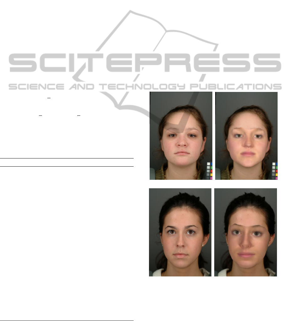
(a) (b)

Figure 1: Example results of the GA face ﬁtting algorithm.

The left column shows the original subjects the right col-

umn the rendered shape estimation that approximately min-

imises the cost function C. The right most image shows the

ﬁnal result of the algorithm.

GRAPP 2012 - International Conference on Computer Graphics Theory and Applications

118

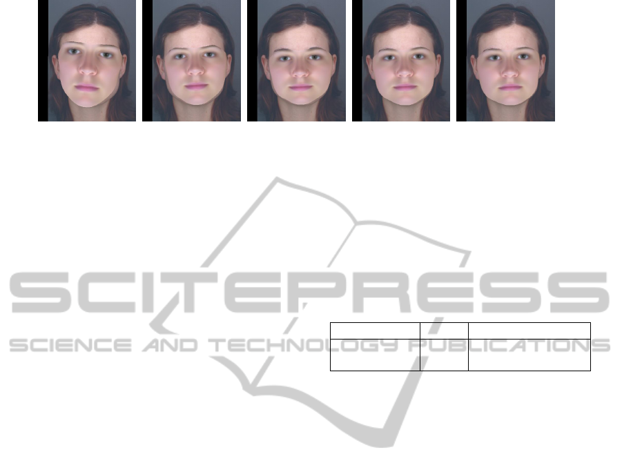
(a) 1

iteration. (b) 3

iteration. (c) 5

iteration. (d) 11

iteration. (e) 28

iteration.

Figure 2: The progress of the Genetic Algorithm in ﬁtting to an example face. Each image shows the best sample from the

indicated iteration.

Shape estimation of each of the 43 subjects was

carried out using both the Genetic-Algorithm method,

outlined above, and using a Taylor-Series gradient de-

scent method similar to (Blanz and Vetter, 1999). For

the Taylor-Series method the faces where initialized

by hand, placing a Morphable Model in the average

conﬁguration in the location on the face that most

closely matched the subjects own face. To overcome

the windowing problem we used a multi-scale ﬁtting

strategy.

Results of ﬁtting using our GA algorithm are

shown in ﬁgures 1 and 3.

In order to get some empirical measures we would

ideally like to have a three-dimensional face model

that exactly matches the photographic image for com-

parison. As we have no access to such models we

opted for a feature point matching strategy. Each

of the 43 photographic images were hand delineated,

marking out clear feature points, e.g. corner of eyes,

mouth, chin etc. Identical landmarks were found on

the Morphable Model, and appropriate shape updates

found such that the landmarks were appropriately ad-

justed when the Morphable Models parameters were

updates. When ﬁtting, either by the Taylor-series

method or the Genetic Algorithm, is completed the

landmarks are updated to match the Morphable Model

and projected onto the two-dimensional image. Each

landmark is compared with its corresponding hand-

placed landmark to determine the accuracy of the ﬁt-

ting in an L

, least squares sense.

∑

− M[ˆs

∑

j=1

i, j

(9)

Here l

is the 2D position of the i

hand-placed land-

mark. ˆs

denotes the position in the 3D shape average

and s

, i the shape update of the i

landmark in the j

principal shape component. M is a linear transform

from 3D to 2D built using the camera parameters.

Table 1 shows the results of ﬁtting to 43 example

images using both the Taylor-Series and Genetic Al-

gorithm methods. From these results we can see that

the GA method offers a clear improvement over the

Taylor-Series method, the difference is signiﬁcant to

p=0.005, using a single-tailed paired t-test.

Table 1: Average error from template ﬁtting computed as

mean squared difference in pixels between landmark pairs.

The images are 378 by 478 pixels. The results are averaged

across 43 ﬁtted images.

Method Mean Standard Deviation

Taylor-Series 44.0 12.9

GA 38.8 4.5

6 CONCLUSIONS

Previous authors have either evaluated the results by

visual inspection or by using the algorithm to identify

an individual from a set of images (Romdhani et al.,

2002; Patel and Smith, 2009). As far as we are aware

we the ﬁrst to have attempted to evaluate the accuracy

of the ﬁtting independently of the cost function, albeit

limited to 2D projection rather than using a speciﬁc

target model.

The algorithm described offers a clear improve-

ment over the simple Taylor-Series method. The Ge-

netic Algorithm is able to reasonably accurately esti-

mate the shape of the face without guidance by fea-

ture landmarks or other form of initialization. We be-

lieve this offers a signiﬁcant improvement over cur-

rent techniques as the method can be applied easily to

large data-sets. One drawback of the algorithm that

is worth mentioning is the speed. The average time

taken for each subject in our set was 18.4 minutes

on a 2.4GHz Intel(R) Core(TM)2 CPU. Gradient de-

scent methods are signiﬁcantly faster, taking an aver-

age of 4.7 minutes each. Although slower our method

is more accurate than the Taylor-Series method. The

standard deviation of the errors is signiﬁcantly larger

for the Taylor-Series method as this method produces

highly inaccurate ﬁts in a number of cases, whereas

the GA method is more consistent.

A GENETIC ALGORITHM FOR FACE FITTING

119

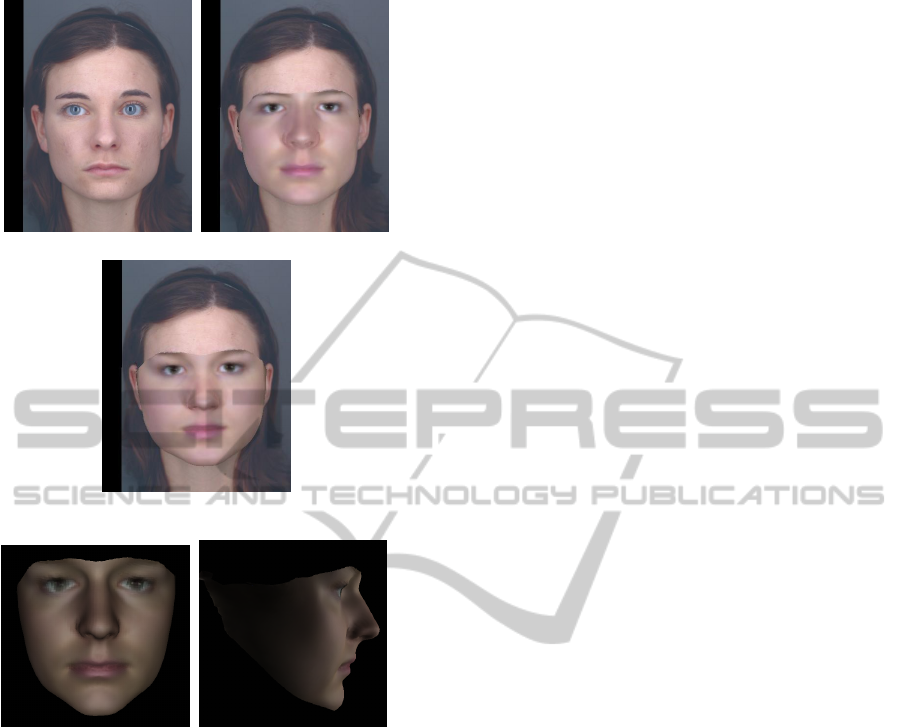
(a) Original image. (b) GA ﬁtted image.

age.

(d) Model only: front

view.

(e) Model only: proﬁle

view.

Figure 3: Example results from the face ﬁtting algorithms.

The top-left image shows the target face image for one of

the subjects. The top right image is the result of the Ge-

netic Algorithm applied to the target image. The middle

row shows the results of ﬁtting using the Taylor-Series al-

gorithm for comparison. On the bottom row the models pro-

duced by the Genetic Algorithm are shown in both full-face

(left) and proﬁle (right) views.

Rather than implement exactly some of the state-

of-the-art techniques we have used a simpliﬁed ver-

sion that distils the various algorithms down to their

essence as iterative gradient descent methods. Some

of the methods such as (Romdhani and Vetter, 2003)

and (Xiao et al., 2004) which attempt to exchange

accuracy for speed are not considered as accuracy is

our main aim. At the other end of the spectrum the

multi-features ﬁtting strategy of Romdhani’s thesis

uses many different error metrics in combination to

produce a face model (Romdhani, 2005). We have

not attempted use all of these metrics in our compar-

ison, however we believe that they are likely to ex-

hibit many of the same problems as the Taylor-Series

method. This is due to the problems of local-minima

and errors in derivative calculation, a problem inher-

ent in gradient descent techniques. It is also worth

noting that both Romdhani’s algorithm (Romdhani,

2005) and (Blanz and Vetter, 1999) both rely on man-

ual placement of landmarks on each face image both

initialise and to guide the ﬁtting. In this respect our

method provides a clear advantage in that no land-

mark placement is required.

REFERENCES

Baker, S. and Matthews, I. (2004). Lucas-kanade 20 years

on: A unifying framework. International Journal of

Computer Vision, 56(1):221 – 255.

Blanz, V. and Vetter, T. (1999). A morphable model for

the synthesis of 3d faces. In SIGGRAPH ’99: Pro-

ceedings of the 26th annual conference on Computer

graphics and interactive techniques, pages 187–194,

New York, NY, USA. ACM Press/Addison-Wesley

Publishing Co.

Cootes, T. F., Edwards, G. J., and Taylor, C. J. (1998). Ac-

tive appearance models. Lecture Notes in Computer

Science, 1407:484–.

Faggian, N., Paplinski, A. P., and Sherrah, J. (2008). 3d

morphable model ﬁtting from multiple views. In FG,

pages 1–6. IEEE.

Luke, S. (2009). Essentials of Metaheuris-

tics. Lulu. Available for free at

http://cs.gmu.edu/∼sean/book/metaheuristics/.

Moghaddam, B., Lee, J., Pﬁster, H., and Machiraju, R.

(2003). Model-based 3d face capture with shape-

from-silhouettes. In In IEEE International Workshop

on Analysis and Modeling of Faces and Gestures,

page pages.

Patel, A. and Smith, W. A. P. (2009). Shape-from-shading

driven 3d morphable models for illumination insensi-

tive face recognition. In BMVC. British Machine Vi-

sion Association.

Romdhani, S. (2005). Face Image Analysis using a Multi-

ple Feature Fitting Strategy. PhD thesis, University of

Basel.

Romdhani, S., Blanz, V., and Vetter, T. (2002). Face iden-

tiﬁcation by ﬁtting a 3d morphable model using linear

shape and texture error functions. In Computer Vi-

sion – ECCV’02, volume 4, pages 3–19, Copenhagen,

Denmark.

Romdhani, S. and Vetter, T. (2003). Efﬁcient, robust and

accurate ﬁtting of a 3d morphable model. In 9th IEEE

International Conference on Computer Vision (ICCV),

pages 59–66.

Xiao, J., Baker, S., Matthews, I., and Kanade, T. (2004).

Real-time combined 2d+3d active appearance models.

In Proceedings of the IEEE Conference on Computer

Vision and Pattern Recognition, volume 2, pages 535

– 542.

GRAPP 2012 - International Conference on Computer Graphics Theory and Applications

120