A SIMPLE DERIVATION TO IMPLEMENT TRACKING

DISTRIBUTIONS

Wei Yu, Jifeng Ning, Nan Geng and Jiong Zhang

College of Information Engineering, Northwest A&F University, No.22 Xinong Road, Yangling, China

eywords:

Tracking, Euler-Lagrange, Active Contours, Level Set.

Abstract:

We present a simple and straightforward derivation to implement active contours for tracking distributions

(Freedman and Zhang, 2004) and its improvement, i.e., distribution tracking through background mismatch

(Zhang and Freedman, 2005). In the original work, two steps are performed in order to derive the tracking

evolution equations. In the ﬁrst step, curve ﬂows are derived using Green’s Theorem, and in the second

step level set method is used to implement the curve ﬂows, which seems to be somewhat complex. In our

implementation, tracking evolution equations are derived directly by using variational theory. This is useful

to understand the tracking method better. The ﬁnal tracking evolution equations are identical to the previous

work (Freedman and Zhang, 2004; Zhang and Freedman, 2005).

1 INTRODUCTION

Determining the location of an object contour is an

important research topic in the ﬁeld of object track-

ing. Tracking methods based on level set theory have

received extensive attention (Freedman and Zhang,

2004; Zhang and Freedman, 2005; Bibby and Reid,

2008; Zhou et al., 2007; Prisacariu and Reid, 2011;

Cremers, 2006; Fussenegger et al., 2006; Allili and

Ziou, 2007) because level set method can implicitly

represent almost any kind of contour and evolve an

active contour naturally.

In the paper (Freedman and Zhang, 2004), authors

devise trackers using distribution distances with three

criteria, Kullback-Leibler distance, Bhattacharyya

measure, and self-developed “simple criterion”. To

extremize distribution distances, ﬁrst, they propose a

proposition by converting a distribution distance from

an area integral to a parameterized curve integral us-

ing Green’s Theorem and calculus of variations which

is very sophisticated. The representation of a parame-

terized curve is in a two dimensional space. So knowl-

edge of differential geometry is required in this de-

duction. After the ﬁrst step, a curve evolution equa-

tion is attained using the gradient method. Finally,

implementation of the curve evolution function uses

the level set method to attain the tracking evolution

function. So the curve evolution is just an intermedi-

ate product and a tool for deduction. But this makes

the deduction hard to be understood by readers. In

the paper (Zhang and Freedman, 2005), a background

density mismatching term is added to the original

equation (Freedman and Zhang, 2004). Although the

principle of background density mismatching term is

similar to that of foreground density matching term, it

allows the algorithm utilise more information so that

it increases the robustness further.

In this paper, we present a new way to deduce a

level set evolution equation without introduction of

the curve ﬂow. This is a really simple method since

it only uses the knowledge of variational theory. Fur-

thermore, this method can calculate a tracking evo-

lution equation directly which reduces the difﬁculty

of understanding the algorithm of tracking distribu-

tions. Although the derivation methods of Daniel

Freedman’s and ours are different, the ﬁnal tracking

evolution equations are the same.

2 BRIEF INTRODUCTION TO

TRACKING DISTRIBUTIONS

2.1 Density Matching Criteria

In (Freedman and Zhang, 2004), Daniel Freedman

et al. propose a new level set based tracking algo-

rithm which ﬁnds the object of interest using fore-

ground match. The tracker aims at ﬁnding the region

ω in a given image such that the sample distribution

351

Yu W., Ning J., Geng N. and Zhang J..

A SIMPLE DERIVATION TO IMPLEMENT TRACKING DISTRIBUTIONS.

DOI: 10.5220/0003816603510354

In Proceedings of the International Conference on Computer Vision Theory and Applications (VISAPP-2012), pages 351-354

ISBN: 978-989-8565-04-4

 2012 SCITEPRESS (Science and Technology Publications, Lda.)

(sample probability density) P

most closely matches

the corresponding model distribution (model proba-

bility density) P

std

. Daniel Freedman (Freedman and

Zhang, 2004) veriﬁes three criteria. In the follow-

ing text, we introduce the algorithm (Freedman and

Zhang, 2004) with Kullback-Leibler distance since

this criterion is the simplest one to implement track-

ing distributions and this criterion is also used in the

paper (Zhang and Freedman, 2005).

Consider a given image I to be a mapping from

Ω ⊆ R

in a plane coordinates system to y which could

be an intensity, color vector and so on. The current

sample probability density (e.g., RGB histogram) of

a region of interest is denoted by P

(y) where ω ⊆ Ω

denotes the region of interest in the image.

Thus, a sample probability density P

(y) is given

(y) =

K(y− I(x)) dx

N(y;ω)

A(ω)

(1)

where K (·) is an n-dimensional function, e.g., for

RGB histogram, n = 3 (RGB vector).

K(a) =

(

1 a =

−→

0 otherwise

(2)

A(ω) is the area of the region ω and N (y, ω) de-

notes the number of pixels of y in the region ω.

For Kullback-Leibler distance:

D(ω) =

std

(y)log



std

(y)



dy (3)

For Bhattacharyya measure:

D(w) =

std

(y) p

(y)dy (4)

It is clear to see that the more closely they match,

the smaller the Kullback-Leibler distance is and the

bigger the Bhattacharyya measure is. So the object of

tracking turns to extremizing D.

2.2 Curve ﬂow

In order to attain the extremal, how to evolve the ac-

tive contours is taken into account. First, a proposi-

tion is proposed as follows:

Proposition: Let ω be an elementary region of R

let c = ∂ω be its boundary, and let Γ(ω) =

µ(x) dx,

where µ is C

. Additionally, let

δΓ

δc

be a 2-vector

whose i

component is the variational derivative

δΓ

δc

assuming a particular parameterization for c. Then

there exists a parameterization of c for which

δΓ

δc

∝ µ(c)~n (5)

where~n is the normal to c.

This proposition is used to calculate curve ﬂows.

Taking the Kullback-Leibler Flow for example,use

the above proposition to calculate

δD

δc

δD

δc

(I(c)) − P

std

(I(c))

N (I(c))

~n (6)

Attain the gradient descent ﬂow using the method

of steepest descent:

∂c

∂t

= −

δD

δc

std

(I (c)) − P

(I(c))

N(I (c))

~n (7)

For Bhattacharyya measure, tracking turns to

maximising D(ω). In a similar way, attain Bhat-

tacharyya gradient ascent ﬂow:

∂c

∂t

δD

δc

2A(ω)

std

(I(c))

− D(ω)

~n (8)

To increase robustness, background density mis-

matching is introduced (Zhang and Freedman, 2005).

Background density mismatching is to maximise the

disparity of probability density between the region

of interest and the background Ω\ω. Therefore, a

curve ﬂow becomes a combination ﬂow based on both

background-mismatching and foreground-matching.

2.3 Implementation with Level Set

Then these ﬂows are implemented using the level set

framework (Osher and Sethian, 1988) for its unparal-

leled advantages in topology.

3 OUR METHOD

In this part, we take Kullback-Leibler distance for ex-

ample to present our deduction.

3.1 Implementation of Energy with

Level Set

In level set theory, the boundary of a region of inter-

est is a curve c which is represented in 3-dimension

space. One more dimension ingeniously allows au-

tomatically topological changes, such as merging and

breaking.

VISAPP 2012 - International Conference on Computer Vision Theory and Applications

352

Let ω ⊆ R

be a region of interest in a given image.

Then the curve c (the boundary of ω, i.e., c = ∂ω) is

represented as the zero level set of a scalar Lipschitz

continuousfunction φ : R

→ R. The levelset function

φ is usually deﬁned as a signed distance function for

the sake of stability.

φ(x) =











> 0 inω

< 0 inΩ\ω

= 0 on∂ω

(9)

where x ∈ Ω ⊆ R

in a plane coordinates system of a

given image.

In order to represent above equations by the level

set function, we need to introduce the Heaviside func-

tion H:

H {z} =

(

1 z ≥ 0

0 z < 0

(10)

Thus the level set formulation of equation (1) is:

(y) =

Ω

K (y− I(x))H (φ)dx

Ω

H (φ)dx

(11)

In our method, equation (3) is referred to as an

energy functional. Minimising this energy is equiv-

alent to ﬁnding a region which represents the closest

distribution as the model distribution (i.e., prior dis-

tribution). Then equation (3) can be implemented by

level set framework:

E (φ) =

∑

std

(y)log





std

(y)

Ω

K(y−I(x))H(φ)dx

Ω

H(φ)dx





(12)

Equation (12) is a fraction-type energy functional

for level set which is different from classic equations

(Chan and Vese, 2001; Vese and Chan, 2002; Li et al.,

2007; Zhang et al., 2010).

3.2 Euler-Lagrange Differential

Equation

Calculus of variations (Wei-chang, 1980) is a com-

mon tool to search for a function that minimizes a

certain functional. The Euler-Lagrange differential

equation is the fundamental equation of calculus of

variations.

E (φ) is a functional and we want to ﬁnd the φ min-

imizing E (φ). When E (φ) reaches its extreme, the

segmentation gets the ideal result ( The probability

density of the region φ ≥ 0 is the same as the model

probability density ). A necessary condition for φ to

yield the minimum of E is : δE = 0, where δ is the

ﬁrst variation of E. In terms of the algorithms of cal-

culus of variations, we have:

δE = −

∑

std

(y)

δP

(y)

(13)

δP

(y) =

A(ω) δN (y;ω) − N (y;ω) δA(ω)

A(ω)

(14)

So, we attain:

δE = −

∑

std

(y)

N (y;ω)

δN (y;ω)−

std

(y)

A(ω)

δA(ω) (15)

where

δN(y;ω) =

Ω

K (y− I(x))δ(φ)δφdx (16)

δA(ω) =

Ω

δ(φ) δφdx (17)

and δ(φ) is the Dirac delta function δ(z) =

H (z) ,

δφ is the ﬁrst variation of φ.

Combine these equations (13)-(17) above and take

account of the arbitrariness of δφ, then we get the

Euler-Lagrange differential equation:

(I(x)) − P

std

(I (x))

N(I (x), ω)

δ(φ(x)) = 0 (18)

So gradient descent with respect to the Euler-

Lagrange differential yields the following evolution:

∂φ(x)

∂t

std

(I (x)) − P

(I(x))

N (I(x), ω)

δ(φ(x)) (19)

We also calculate the evolution equation of the en-

ergy model using Bhattacharyya measure which is the

same as the results of the work (Freedman and Zhang,

2004; Zhang and Freedman, 2005).

In Bhattacharyya criterion-based model, we attain

the Euler-Lagrange differential equation as follows:

2A(ω)

std

(I(x))

− D(ω)

δ(φ(x)) = 0 (20)

and its tracking evolution equation is:

∂φ

∂t

2A(ω)

std

(I(x))

− D(ω)

δ(φ(x)) (21)

So comparing the equations above, equations (18)

and (20) correspond to equations (7) and (8). Af-

ter equations (7) and (8) is implemented by level set

method, two deductions get the same results as equa-

tion (19) and equation (21).

A SIMPLE DERIVATION TO IMPLEMENT TRACKING DISTRIBUTIONS

353

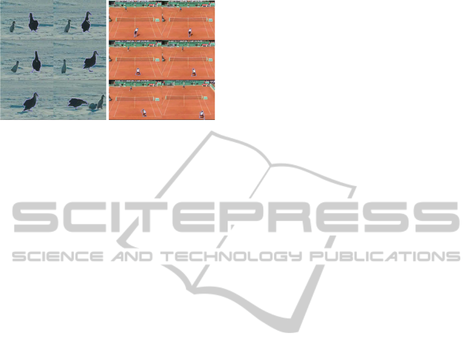
Figure 1: Left: Tracking results of bird sequence with

Kullback-Leibler criterion. Frame 20, 40, 60, 80, 100

and 120 are displayed.(resolution of 320x240, 25 FPS)

Rright: Tracking results of player sequence with Kullback-

Leibler criterion. Frame 2, 13, 24, 35, 46 and 79 are dis-

played.(resolution of 512x380, 25 FPS)

4 EXPERIMENTAL RESULTS

We used an Intel Core2 E7300 (2.66GHz) machine

to run all our experiments using the algorithm of

distribution tracking through background mismatch

(Zhang and Freedman, 2005). The model distribu-

tions are built as 8-bin RGB histograms out of the bird

and out of the player taken from the ﬁrst frame respec-

tively. We show 2 experimental results in Fig.1. The

results show that this algorithm can evolve the bound-

ary of the tracking object correctly although there ex-

ist large non-rigid deformations.

5 CONCLUSIONS

In this paper, we present a simple way of deduction to

implement two important tracking algorithms (Freed-

man and Zhang, 2004; Zhang and Freedman, 2005)

based on level set theory. Our deduction results are

identical to the previous work (Freedman and Zhang,

2004; Zhang and Freedman, 2005). Further, our evo-

lution equations for level set are deduced in a straight-

forward and direct way. This way of deriving an evo-

lution equation can provide readers with an intuitive

explanation of the foreground density matching algo-

rithm and the background density mismatching algo-

rithm, which helps understand and uses these two al-

gorithms better.

ACKNOWLEDGEMENTS

This work is partially supported by the National

Science Foundation of China (NSFC) under Grant

No.61003151, the Fundamental Research Funds for

the Central Universities under Grant No.QN2009091,

Northwest A&F University Research Foundation un-

der Grant No.Z111020902 and the International Co-

operation Foundation of Northwest A&F University.

REFERENCES

Allili, M. S. and Ziou, D. (2007). Active contours for video

object tracking using region, boundary and shape

information. Signal, Image and Video Processing,

1(2):101–117.

Bibby, C. and Reid, I. (2008). Robust real-time visual track-

ing using pixel-wise posteriors. Proceedings of the

European Conference on Computer Vision (ECCV)

2008, page 831–844.

Chan, T. F. and Vese, L. A. (2001). Active contours with-

out edges. IEEE Transactions on Image Processing,

10(2):266–277.

Cremers, D. (2006). Dynamical statistical shape pri-

ors for level set-based tracking. IEEE Transactions

on Pattern Analysis and Machine Intelligence, page

1262–1273.

Freedman, D. and Zhang, T. (2004). Active contours for

tracking distributions. IEEE Transactions on Image

Processing, 13(4):518–526.

Fussenegger, M., Deriche, R., and Pinz, A. (2006). Mul-

tiregion level set tracking with transformation invari-

ant shape priors. Proceedings of Asian Conference on

Computer Vision 2006, page 674–683.

Li, C., Kao, C., Gore, J., and Ding, Z. (2007). Implicit ac-

tive contours driven by local binary ﬁtting energy. In

2007 IEEE Conference on Computer Vision and Pat-

tern Recognition, page 1–7.

Osher, S. and Sethian, J. A. (1988). Fronts propagating

with curvature-dependent speed: algorithms based on

Hamilton-Jacobi formulations. Journal of computa-

tional physics, 79(1):12–49.

Prisacariu, V. and Reid, I. (2011). Nonlinear shape man-

ifolds as shape priors in level set segmentation and

tracking.

Vese, L. A. and Chan, T. F. (2002). A multiphase level set

framework for image segmentation using the mum-

ford and shah model. International Journal of Com-

puter Vision, 50(3):271–293.

Wei-chang, Q. (1980). Calculus of variations and ﬁnite el-

ement [M]. Beijing: Science Press.

Zhang, K., Song, H., and Zhang, L. (2010). Active contours

driven by local image ﬁtting energy. Pattern Recogni-

tion, 43(4):1199–1206.

Zhang, T. and Freedman, D. (2005). Improving perfor-

mance of distribution tracking through background

mismatch. IEEE transactions on pattern analysis and

machine intelligence, page 282–287.

Zhou, X., Hu, W., and Li, X. (2007). An adaptive shape

subspace model for level set-based object tracking.

In Subspace 2007. Workshop on Asian Conference on

Computer Vision, page 9–16.

VISAPP 2012 - International Conference on Computer Vision Theory and Applications

354