
CODED PIXELS
Random Coding of Pixel Shape for Super-resolution
Tomoki Sasao
1
, Shinsaku Hiura
2
and Kosuke Sato
1
1
Graduate School of Engineering Science, Osaka University
1-3 Machikaneyama-cho, Toyonaka, Osaka, 560-8531, Japan
2
Graduate School of Information Sciences, Hiroshima City University
3-4-1 Ozuka-Higashi, Asa-Minami-Ku, Hiroshima, 731-3194, Japan
Keywords:
Super-resolution, Image Sensor, Richardson-Lucy Deconvolution.
Abstract:
In this paper, we propose a technique to improve the performance of super-resolution by changing the effec-
tive shape of each pixel on the image sensor. Since the sampling of the incoming light by the usual image
sensors is not impulse-shaped but rectangular, the high spatial frequency component of the latent image is lost
through the integration effect of the pixel area. Therefore, by spraying black powder onto the image sensor we
give each pixel shape a random code, which jointly aggregates the latent information of the observed scene.
Experimental results show that the proposed random code greatly improves the quality of the reconstructed
image.
1 INTRODUCTION
In recent years, multi-frame super-resolution tech-
niques have been intensively studied to acquire a
high-resolution image from a sequence of images.
However, the resolution of the output image is lim-
ited even if we can use an infinite number of low-
resolution input images (Tanaka and Okutomi, 2005).
This limitation stems from the integration effect of
each pixel shape, which determines the PSF (point
spread function), and then, the image blurred by the
PSF is observed by many samples. The shape of the
pixel should therefore, be designed to retain the latent
informationof the scene. We thus propose the concept
of random coding of the pixel shape to improve the
performance of super-resolution. In the spatial fre-
quency domain, a random pixel shape has no evident
weak point of low response. Moreover, the random
coding is suitable for various camera motions.
Since it is not easy to fabricate custom image sen-
sors with random pixel shapes, we use black powder
spread on the image sensor. The arrangement of the
particles of powder is impossible to control, and thus
we also propose a fast technique to determine the sen-
sitivity distribution of each pixel using a high reso-
lution LCD display. In this paper, we first describe
the implementation of the sensor sprinkled with black
powder using the method to determine the arrange-
ment of each particle, and then we present our exper-
imental results.
2 RELATED WORK
One of the most relevant studies is Penrose Pixels pro-
posed by Ben-Ezra et al. (Ben-Ezra et al., 2007). The
authors argued that their Penrose tiling pattern is bet-
ter for super-resolution than a square tiling because
the pattern is perfectly aperiodic. However, the ar-
rangement of the pixel position is not essential for the
performance of multi-frame super-resolution since we
have denser samples with an infinite number of ran-
domly translated images. However, the shape of the
pixel does affect the performance of super-resolution,
because the integration of the incoming light by each
pixel acts as a low-pass filter for the latent image. In
other words, we observe the sampled values of the
blurred image by pixel integration, and the number
of input images directly corresponds to the density of
the sampling. From this point of view, Penrose tiling
is not optimal because it has only ten pixel shape vari-
ations including rotation.
Tanaka et al. (Tanaka and Okutomi, 2005) also
discussed the problem of the theoretical limit of
super-resolution due to the pixel shape if we could
use an infinite number of input images. In their paper,
168
Sasao T., Hiura S. and Sato K..
CODED PIXELS - Random Coding of Pixel Shape for Super-resolution.
DOI: 10.5220/0003817001680175
In Proceedings of the International Conference on Computer Vision Theory and Applications (VISAPP-2012), pages 168-175
ISBN: 978-989-8565-03-7
Copyright
c
2012 SCITEPRESS (Science and Technology Publications, Lda.)
they pointed out that a square pixel has zero response
for some spatial frequencies as shown in Figure 1. On
the other hand, a Gaussian PSF is not suitable for a
high magnification ratio because it loses the high spa-
tial frequency components. From their conclusions,
it is evident that the PSF of the pixel shape should
retain the high spatial frequency components without
zero response. However, since their theory assumes a
space-invariant PSF, the potential for a space-varying
PSF with assorted pixel shapes has not been investi-
gated.
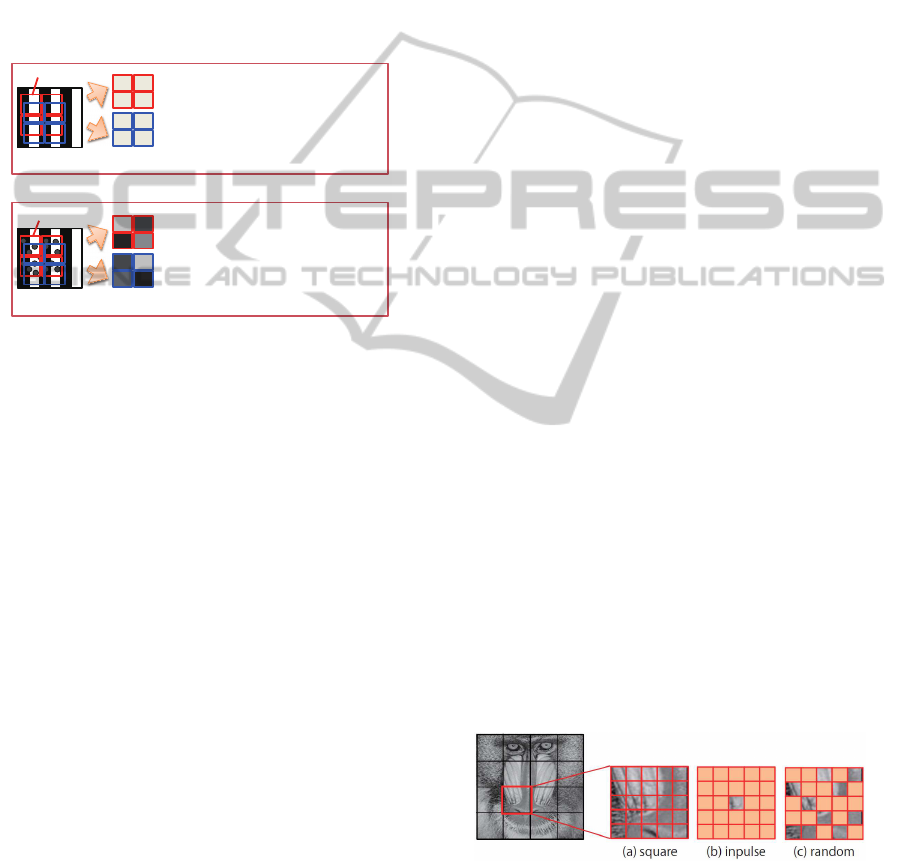
!
Figure 1: Advantages of random pixel shapes. If we capture
a striped pattern with pitch equal to the width of each pixel,
the information of the pattern is never discovered by the
sensor. Contrarily, if we use a randomly coded pixel shape,
the values from the pixels differ. Moreover, the change in
values during the translation of the camera gives more in-
formation to recover the detail of the scene.
Of course, type of algorithm for super-
resolution(SR) also matters to the quality of the
reconstructed image. In general, SR algorithms can
be classified into single-frame and multi-frame SR.
Since the former one is obviously ill-posed, some
sort of prior knowledge about the latent image is
necessary. Additionally, even for the latter case,
the use of priors is also very effective to obtain
low-noise and sharp results. In mathematics, the
reconstruction of latent image which well satisfies
the statistical model of prior is classified to MAP
(Maximum A Posteriori) estimation, and algorithms
to find the solution have been very well investigated
(Hardie et al., 1997). In addition, since pixel values
in any images are always non-negative, a simple
iterative algorithm called NMF (Non-negative Matrix
Factorization) has been proposed (Lee and Seung,
2001). In this paper, we never discuss about pros and
cons of such algorithms. In experiments, we simply
applied MAP, NMF and modified version of RL
(Richardson, 1972) algorithms for the reconstruction
of latent images.
3 CODED PIXELS
In this section we introduce the idea of improving
the quality of a high-resolution image reconstructed
from multiple low-resolution images. As shown in
Figure 1, a square-shaped pixel on the usual image
sensor loses information of the input signal at a cer-
tain spatial frequency. In other words, the output of
the pixel has a zero value for a signal of which the
period is the same as the width of the integration, and
it is impossible to reconstruct the information of the
frequency. Note that all the pixels of the usual image
sensor have the same shape of light sensitivity, and
the lost frequency is common to all the pixels. On
the other hand, a coded pixel is essentially broadband
in spatial frequency, and moreover, a different code
for each pixel suppresses the ill-conditioned case by
using multiple input images.
For a more specific discussion, let us consider the
three types of codes shown in Figure 2. As described
above, the square pixel (a) loses some of the infor-
mation of the latent image. Contrarily, the impulse-
shaped light sensitive pattern (b) is theoretically ideal
because the spatial frequency of the impulse is broad-
band. However, this pattern is susceptible to a variety
of noise in the actual system because the transmis-
sion of the incoming light is very small. Fortunately,
the frequency response of the random code (c) varies
for each pattern, and in some cases it could have zero
response at a certain frequency. However, such ill-
conditionedfrequencyis not common to the other pix-
els, and more input images may offer better results.
Another advantage of the random pattern is the
independence from the motion of the image. If the
camera motion is pure horizontal translation, both the
square pixel (Figure 2(a)) and the impulse sampling
(Figure 2(b)) offer no super-resolution effect for the
vertical axis. On the other hand, the random pat-
tern has no ill-conditioned case for image motion, and
even the vertical spatial frequency benefits from the
rewards through the horizontal motion of the scene.
Figure 2: Differences in information provided by the code.
We can validate the effect of the random pixel
shape through simulation, and in fact these results are
shown later. However, since it is not easy to fabricate
image sensors with arbitrary pixel shapes, we sprinkle
fine black powder onto the image sensor to encode a
CODED PIXELS - Random Coding of Pixel Shape for Super-resolution
169
random pixel shape. This method raises some prob-
lems. In fact, current image sensors have so many
pixels that it is not easy to find black powder with par-
ticles sufficiently smaller than the pixel size. More-
over, the arrangement and shape of the particles must
be determined, because the arrangement of the parti-
cles is impossible to control. We describe a method to
estimate the effective sensitivity distribution of each
pixel in the next section.
3.1 Random Coding by Sprinkling
Black Powder
Random coding is applied by sprinkling fine black
powder on an image sensor. However, since the pixel
size of current image sensors is so small, it is not easy
to find suitable powder for sprinkling. In fact, the
pixel size of the camera we used (Lumenera company,
Lu125) is 6.7 µm * 6.7 µm. The powder used for the
coding is black toner for laser printers. Using a micro-
scope, we determined the diameter of each particle to
be about 6µm. Therefore, we combined several pixel
values to form a large virtual pixel in the experiments.
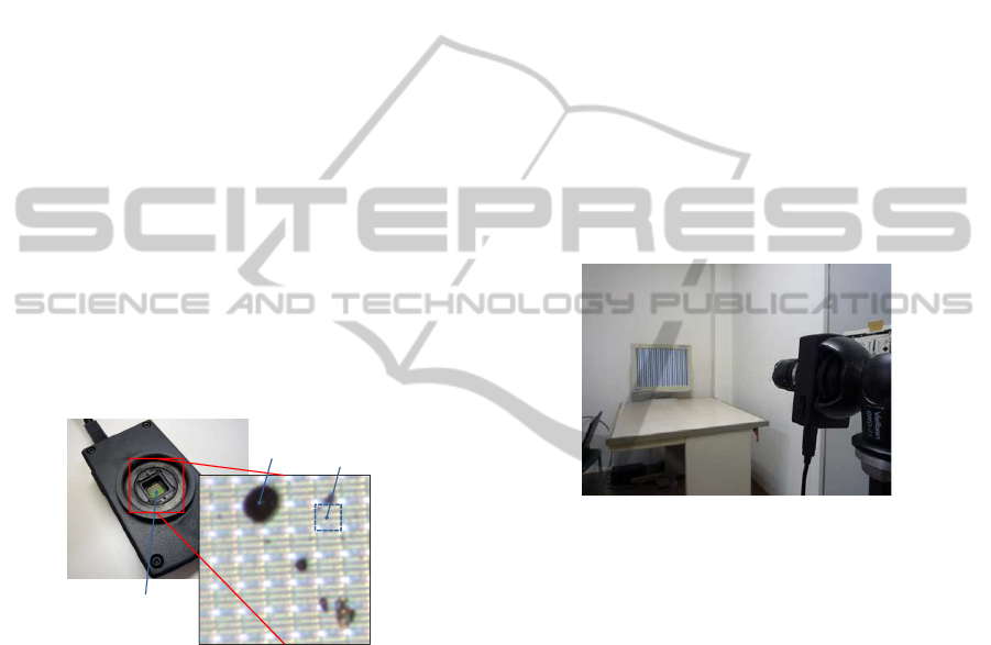
Figure 3 shows the toner on the image sensor as ob-
served with a microscope.
1 pixel
Toner
Image sensor
Figure 3: Toner on the image sensor.
3.2 Identification of Random Codes
One approach for identifying the arrangement of the
particles of black powder is directly observing the im-
age sensor using a microscope, as shown in Figure 3.
However,registeringthe pixel positions is difficult be-
cause the contrast of the pixels on the image sensor is
very low. Moreover, the arrangement of black toner
does not always correspond to the distribution of the
light sensitivity of each pixel. Therefore, we iden-
tified the sensitivity distribution of each pixel using
the captured image of the sensor itself with controlled
scene images. The principle of the identification is as
follows.
(1) Place a very small point light source in the scene,
and then take an image with the contaminated im-
age sensor. The intensity values of the pixels cor-
responding to the position of the light source will
increase, if the point light is not blocked by parti-
cles.
(2) Repeat capturing images with a slight translation
of the point light source.
(3) The distribution of the light sensitivity of each
pixel according to the position of the light source
is identified.
Obviously, the resolution of the distribution of
light sensitivity depends on the pitch of the transla-
tion of the point light source. This means that a more
accurate identification will take longer to capture so
many images when using a single light source, and
thus we use a technique to shorten the measurement
time by using multiple light sources. Actually, for the
identification, we use an LCD display as an array of
point light sources. As shown in Figure 4, the display
is placed in front of the camera.
Figure 4: Relation of camera and display.
As described above, we can use multiple light
sources to shorten the measurement time. In this case,
it is necessary to distinguish which light source affects
each pixel. In other words, each pixel should receive
light from only one particular light source. There-
fore, the space between two neighboring light sources
should be greater than the width of light sensitivity of
each pixel as shown in Figure 5. The correspondence
between a pixel of the camera and the display is de-
termined using the Gray-code measurement method.
The process to determine the light sensitivity of each
pixel is given below.
(1) Vertical and horizontal stripes of Gray-code are
displayed on the LCD panel, and captured by the
image sensor. In the process, each pixel is associ-
ated with coordinates on the LCD panel.
(2) The periodic dot pattern depicted in Figure 5 is
displayed on the LCD panel, and an image is cap-
tured.
(3) One lighting pixel on the LCD panel is deter-
mined by selecting the nearest lighting pixel to the
coordinates corresponding to the camera pixel.
VISAPP 2012 - International Conference on Computer Vision Theory and Applications
170

(4) The sensitivity from the point light source to the
camera pixel is recorded.
(5) The dot pattern is shifted pixel by pixel, and then
steps (2) to (4) are repeated.
Camera pixel
Display pixel
Point
light
Figure 5: Projection of the dot pattern.
d
i
u
j
p
ij
=
*
*
*
*
*
*
*
*
*
*
*
*
*
*
*
*
*
*
0
0
.
.
.
l
2
pixels
Figure 6: Sparse matrix representation of light sensitivity
distribution.
Finally, we obtain the light sensitivity distribu-
tion of each pixel. The distribution obtained by this
process is represented as shown in Figure 6. In the
figure, vector d
i
denotes the pixel value of the cam-
era, while u
j
is the intensity distribution on the LCD
panel. Since the resolution of the LCD panel is higher
than that of the camera, the length of u
j
is longer than
c
i
, and matrix p
ij
describes the relationship between
the LCD panel and the camera. Since the area of light
sensitivity of each camera pixel is so small, matrix
p
ij
is sparse. If the area of light sensitivity of each
pixel on the LCD panel is limited to l × l, the num-
ber of non-zero entries in each row is less than l
2
, as
shown in Figure 6. This characteristic is very useful
not only to shorten the measurementtime as described
above, but also to reduce the memory requirement for
the light sensitivity distribution.
For the super-resolution, vector u
j
corresponds to
the high-resolution latent image, and d
i
is the low-
resolution observed image. Therefore, the resolution
of the LCD panel used to identify the distribution of
particles determines the resolution of the recovered
high-resolution image by super-resolution.
3.3 Shift-varying Richardson-Lucy
Deconvolution
Usually, we assume a shift-invariant PSF for super-
resolution. However, as described above, the codes
given for the camera pixels are not identical to each
other. Therefore, we must deal with a shift-varying
PSF in the super-resolution calculation. Unfortu-
nately, some algorithms and frameworks for decon-
volution are limited to shift-invariant PSFs. For ex-
ample, we cannot use Fourier-transform based decon-
volution techniques such as Wiener filters.
In this section, we present a modification of the
Richardson-Lucy (RL) deconvolution (Richardson,
1972). Originally, RL deconvolution was limited to
shift-invariant PSFs, but a small modification allows
handling the shift-varying case, which includes ran-
dom codes.
The RL algorithm is an iterative method to recon-
struct an original image degraded by a known PSF.
As shown in Figure 6, observed image d
i
can be de-
scribed as
d
i
=
∑
j
p
ij
u
j
(1)
where p
ij
is the PSF, u
j
is the pixel value of the origi-
nal image at pixel index j, and d
i
is the pixel value of
the observed images at sample index i. RL deconvo-
lution reconstructs the latent image u
j
by calculating
the recurrence equations:
u
(t+1)
j
= u
(t)
j
∑
i
d
i
c
i
p
ij
(2)
c
i
=
∑
j
p
ij
u
(t)
j
(3)
Unfortunately, the original RL algorithm is lim-
ited to shift-invariant PSFs, and thus we extend it to
handle the shift-varying case. In the final stage of the
calculation, result u
(t)
j
should converge to the latent
image u
j
, so we can lead the condition
d
i
c
i
= 1 (4)
by comparing Equations 1 and 3. In this case, the
recurrence Equation 2 can be simplified as
u
(t+1)
j
= u
(t)
j
∑
i
p
ij
(5)
at the converged state u
(t+1)
j
= u
(t)
j
. Therefore, it is
necessary to satisfy the following equation
∑
i
p
ij
= 1 (6)
since the reconstructed image u
j
cannot be changed.
However, Equation 6 is not satisfied in the case of
shift-varying PSFs. Therefore, we extend the recur-
rence equation of the RL method as
u
(t+1)
j
= u
(t)
j
∑
i
d
i
c
i
p
ij
∑
i
p
ij
=
1
∑
i
p
ij
u
(t)
j
∑
i
d
i
c
i
p
ij
(7)
to compensate the nonuniform gain of updating the
image.
CODED PIXELS - Random Coding of Pixel Shape for Super-resolution
171

4 SIMULATION EXPERIMENTS
FOR COMPARING CODES
In this section we verify the performance of random
coded pixels with the RL method through simulation.
4.1 Simulation Conditions
The image used in the experiment is shown in Fig-
ure 7. The super-resolution factor is 14× 18, and the
resolution of the input image is very low as shown in
Figure 7(b). The assumed camera motion is horizon-
tal with vertical pixel-wise translation of the original
image. Therefore, each pixel shift on the observed
image is 0.07 of the pixel width and 0.055 of the pixel
height. We used 252 images with different shift val-
ues, and therefore the number of observed samples
and output pixels is the same.
(a) LRI (b) HRI
Figure 7: Original high-resolution latent image (b) and cor-
responding low-resolution input image (a) for the simula-
tion experiment.
We comparedthe five types of codes shown in Fig-
ure 8. We divided each observed pixel into 14*18
subpixels, and set a transmission ratio for each sub-
pixel. Therefore, the size of each subpixel is the same
as the latent image. Figure 8(a) simulates the usual
image sensor filled with 100% square pixels. The
pinhole code (b) can be considered to be an identi-
cal transform from the latent image to the input value.
Codes (c) and (d) are random codes generated by dif-
ferent algorithms. Transmission of code (c) is a con-
tinuous value, whereas code (d) consists of randomly
arranged multi-pinhole codes. Code (e) is a code for
the Gaussian distribution with variance 5.0. The noise
model used in the experiment is additive noise. Since
smaller transmission decreases the pixel values, the
worse the SN ratio becomes. For example, pinhole
code (b) has 252 times larger noise relative to the sig-
nal value than the square pixels (a). We used two
magnitudes of noise in the experiment. The added
noise has a Gaussian distribution with zero mean and
standard deviation of 1.0 and 20.0 for the 8-bit input
images.
(a) full (b) pinhole
(c) rand-all (d) rand-pos
(e) gauss
Figure 8: Codes for each pixel used in the simulation:
(a) square shape of normal image sensor (aperture ratio =
100%), (b) one of 14*18 subpixels open, very small aper-
ture ratio (0.4%) like impulse sampling, (c) transmission
ratio of all sub-pixels is random, not periodic, (d) transmis-
sion ratio of each sub-pixel is 1 or 0, randomly assigned, (e)
transmission ratio has a Gaussian distribution pattern.
4.2 Results
The PSNRs of the reconstructed high-resolution im-
ages with different codes and noise values are shown
in Figure 1. Magnified views of the reconstructed im-
ages are also shown in Table 1. It is clearly shown
that the pinhole code (b) with little noise is the best,
because the capturing process can be considered to be
an identical transform. However, the result for much
noise is the worst, because the sensitivity of the sensor
is very low. The case of full-aperture (a) has the most
light efficiency, however, the result is not at all sharp
for both noise values. In the case of much noise, the
rand-pos code (d) is the best in the PSNR evaluation;
it is also the best in the case of little noise except for
the pinhole code. The appearance of the output im-
age using rand-pos code (d) is also the best as shown
in Figure 1; in particular, the fine detail is very well
reconstructed with less noise than the pinhole code.
5 EXPERIMENTS WITH A REAL
CONTAMINATED SENSOR
We used a real camera without a cover glass and
contaminated with black toner from a laser printer.
First, we show the experimental results of identifying
the arrangement of the particles, and then the results
of super-resolution with several reconstruction algo-
rithms.
VISAPP 2012 - International Conference on Computer Vision Theory and Applications
172
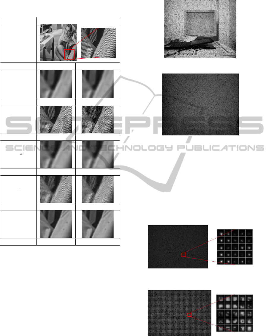
Table 1: Super-resolution simulation results with different
codings of the shape of the light sensitivity of each pixel.
barbara image
target image
gauss noise little noise much noise
full
PSNR 22.372787 22.372758
pinhole
PSNR 48.108994 22.180849
rand all
PSNR 22.515605 22.511611
rand pos
PSNR 25.181091 25.300695
gauss
PSNR 23.85785 23.856232
5.1 Identification of Light Sensitivity
Distribution
The camera used in the experiment is an Lu125
(Lumenera company) without a cover glass on the
sensor. As described above, we found the average di-
ameter of particles of the black toner to be about 6 µ.
Specifications of the equipment used are given below.
• Pixel pitch: 6.7 µm * 6.7 µm
• Resolution of the camera: 1280*1024
• Exposure time: 350 ms
• Resolution of LCD display: 1600*1200
In the experiments, we used a part of the image
sensor as shown in Figure 9. Here, the area of the
LCD panel in the captured image is about 360× 300
Figure 9: Arrangement of LCD panel.
Figure 10: Input image for flat white scene.
pixels. Figure 10 shows an image of white paper taken
with the coded camera. We see that the toner is scat-
tered over the whole image sensor.
Figure 11 shows the results of the identified light
sensitivity distributionof each camera pixel. Since the
size of the pixel is very similar to the size of the toner
particles, it is not clear whether the particle covers the
pixel. Therefore, we combined 3× 3 pixel values into
a single value to form larger virtual pixels, resulting
in an input image size of 120× 100 pixels.
Figure 11: Estimated light sensitivity distribution of an ac-
tual pixel of the sensor with black powder.
Figure 12: Estimated light sensitivity distribution of 3× 3
combined virtual pixels with black powder.
Figure 12 shows the results of the identified light
sensitivity distribution of each virtual camera pixel.
CODED PIXELS - Random Coding of Pixel Shape for Super-resolution
173

Since we use 3× 3 pixels as a single pixel, the iden-
tified light sensitivity has gaps between neighboring
actual gaps. Please note that we never used the raw
independent pixel values, but combined only the in-
tensity. This shows that the method for identifying
light sensitivity works properly. We carried out the
same process for the camera without contamination.
Figure 13 shows the clear shape of the virtual pixels.
Figure 13: Estimated light sensitivity distribution of 3 × 3
combined virtual pixels without black powder.
5.2 Super-resolution with Controlled
Scene Motion
Before we attempted an experiment with unknown
object motion, we carried out an experiment using im-
ages with known motion. We used the light sensitivity
distribution identified in Section 5.1(Figure 12,13).
To capture images with known motion, we used the
display for calibration to show an image to the sensor.
The image on the display was shifted pixel by pixel
to capture images with controlled translation. The ex-
perimental conditions are as follows.
• Translation of each image is known
• Number of input images: 576
• Virtual input image: (120, 100) pixels
• Reconstructed image: (1600, 1200) pixels
The image used in the experiment is a star chart
as shown in Figure 14. Figure 14(a) shows one of the
input images without black powder.
(a) Input image (b) Ground truth
Figure 14: Image used in the experiment and captured im-
age.
Table 2 shows the reconstructed images and quan-
titative evaluation result (PSNR), where INVERSE
denotes the direct solution by calculating the inverse
Table 2: Super-Resolution result by coding the pixel shape.
Chart image
target image
Kind of code @no code@ random code
INVERSE
PSNR 11.858526 13.138333
MAP
PSNR 9.260995 11.755036
NMF
PSNR 11.624983 11.873994
RL
PSNR 10.960783 12.88722
of the light transport matrix p
ij
. MAP and NMF are
the estimation with maximum-a-posteriori and non-
negative matrix factorization algorithms, respectively,
with a smooth edge prior. RL is the modification of
the Richardson-Lucy algorithm described in Section
3.3.
The results show that the random coded sensor al-
ways produces better results for all reconstruction al-
gorithms. In particular, the sensor without random
coding shows lost spatial frequency, but the random
coding suppresses such failure cases for all frequen-
cies.
5.3 Experiment using Real Scene with
Unknown Motion
We performed an experiment to estimate a high-
resolution image from the input image shown in Fig-
ure 15. We used the light sensitivity distribution iden-
VISAPP 2012 - International Conference on Computer Vision Theory and Applications
174
tified in Section 5.1(Figure 12,13). In this experi-
ment, we captured 300 real images using a camera
with arbitrary motion. The motion of the scene was
estimated using a Phase Only Correlation (POC) al-
gorithm (Kuglin, 1975). Since the variation in pixel
sensitivity degrades the accuracy of motion estima-
tion, we used a compensated image. More specifi-
cally, we took a picture of a flat white scene as shown
in Figure 10 as a reference, and then the images of
the actual scene were divided by the reference image.
The compensated image looks clearer with very slight
effects of contamination, so it is better for motion es-
timation.
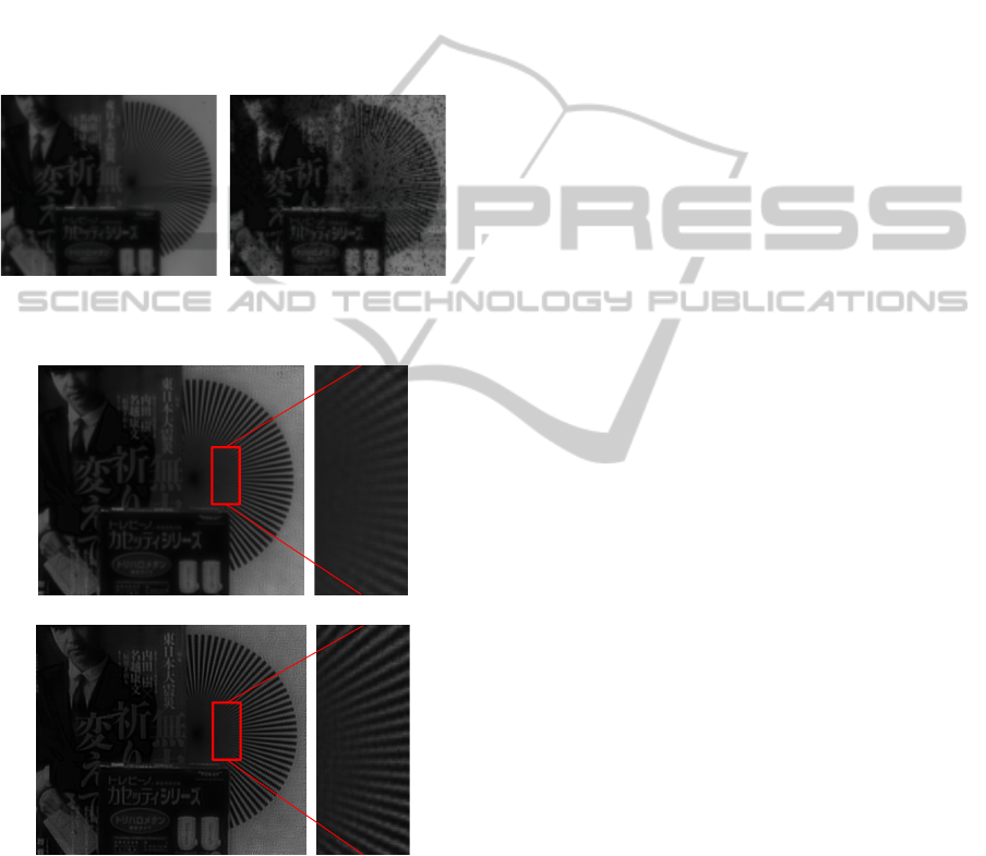
(a) no code (b) random code
Figure 15: Observation image.
(a) no-code
(b) random-code
Figure 16: Super-Resolution results for no-code and
random-code.
Figure 16 shows the results of applying the modi-
fied RL algorithm to the observation images for each
estimated code. Although it is impossible to evaluate
the result quantitatively, it is clear from the results that
the randomly coded sensor is better than the one from
the original sensor.
6 CONCLUSIONS
We focused on the loss of the high frequency com-
ponent caused by the pixel shape of image sensors,
and proposed a random coding for the pixel shape.
In addition, we tried to implement such a device by
sprinkling fine black powder on the image sensor. The
arrangement of black particles was calibrated using
the captured images. The results clearly show that
the coded pixel has advantages for multi-frame super-
resolution. We also argued that constructing a real
Coded Pixel sensor is feasible with current technol-
ogy. Manufacturing the image sensors with randomly
shaped pixels will be a challenge in the future.
ACKNOWLEDGEMENTS
This work was partially supported by Grant-in-Aid
for Scientific Research (B:21300067) and Grant-
in-Aid for Scientific Research on Innovative Areas
(22135003)D
REFERENCES
Ben-Ezra, M., Lin, Z., and Wilburn, B. (2007). Penrose
pixels super-resolution in the detector layout domain.
volume 0, pages 1–8. IEEE 11th International Confer-
ence on Computer Vision.
Hardie, R., Barnard, K., and Armstrong, E. (1997). Joint
map registration and high-resolution image estimation
using a sequence of undersampled images. volume 6,
pages 1621–1633. IEEE.
Kuglin, C. (1975). The phase correlation image alignment
methed. In Proc. Int. Conference Cybernetics Society,
pages 163–165.
Lee, D. and Seung, H. (2001). Algorithms for non-negative
matrix factorization. volume 13, pages 556–562. MIT
Pres.
Richardson, W. (1972). Bayesian-based iterative method of
image restoration. volume 62, pages 55–59. Optical
Society of America.
Tanaka, M. and Okutomi, M. (2005). Theoretical analysis
on reconstruction-based super-resolution for an arbi-
trary psf. volume 2, pages 947–954. IEEE Computer
Society.
CODED PIXELS - Random Coding of Pixel Shape for Super-resolution
175
