DEPTH PERCEPTION MODEL EXPLOITING BLURRING CAUSED

BY RANDOM SMALL CAMERA MOTIONS

Norio Tagawa, Yuya Iida and Kan Okubo

Graduate School of System Design, Tokyo Metropolitan University, Hino-shi, Tokyo, Japan

Keywords:

Depth Perception, Shape from Blurring, Stochastic Resonance, Fixational Eye Movement.

Abstract:

The small vibration of the eye ball, which occurs when we ﬁx our gaze on an object, is called “ﬁxational eye

movement.” It has been reported that this vibration may work not only as a fundamental function to preserve

photosensitivity but also as a clue to image analysis, for example contrast enhancement and edge detection.

This mechanism can be interpreted as an instance of stochastic resonance, which is inspired by biology, more

speciﬁcally by neuron dynamics. Moreover, researches for a depth recovery method using camera motions

based on an analogy of ﬁxational eye movement are in progress. In this study, using camera motions espe-

cially corresponding to the smallest type of ﬁxational eye movement called “tremor.” We have constructed

the algorithms which are deﬁned as a differential form, i.e. spatio-temporal derivatives of successive two im-

ages are analyzed. However, in these methods, observed noise of derivatives causes serious recovering error.

Therefore, we newly examine a method in which a lot of images captured with the same camera motions are

integrated and the observed local image blurring is analyzed for extracting depth information, and conﬁrm its

effectiveness.

1 INTRODUCTION

Camera vibration noise is serious for a hand-held

camera and for many vision systems mounted on mo-

bile platforms such as planes, cars or mobile robots,

and of course for biological vision systems. The com-

puter vision researchers traditionally considered the

camera vibration as a mere nuisance and developed

variousmechanical stabilizations (Oliverand Quegan,

1998) and ﬁltering techniques (Jazwinski, 1970) to

eliminate the jittering caused by the vibration.

In contrast, a new vision device, called the Dy-

namic Retina (DR), which directly takes advantage

of vibrating noise generated by mobile platforms to

enhance spatial contrast (Propokopowicz and Cooper,

1995). Furthermore, for edge detection, the Resonant

Retina (RR) indicating the DR model with the tech-

nique based on stochastic resonance (SR) is proposed

(Hongler et al., 2003). SR can be viewed as a noise-

induced enhancement of the response of a nonlinear

system to a weak input signal, for example bistable

devices (Gammaitoni et al., 1998) and threshold de-

tectors (Greenwood et al., 1999), and naturally ap-

pears in many neural dynamics processes (Stemmler,

1996).

Although DR and RR offer their massive paral-

lelism and the simplicity of their architecture, by con-

sidering especially the enough potential of the cam-

era vibration for depth perception, we have proposed

shape recovery methods using the camera motion

model imitating ﬁxational eye movements (Tagawa

and Alexandrova, 2010), (Tagawa, 2010). These

methods are constructed based on a differential form,

and the gradient method for ”shape from motion”

(Horn and Schunk, 1981), (Simoncelli, 1999), (Bruhn

and Weickert, 2005) is used fundamentally in order

to recover dense depth map with low computational

cost compared with the methods based on correla-

tion matching. The ﬁxational eye movement is clas-

siﬁed into three types as shown in Fig. 1: microsac-

cade, drift and tremor. Here, we focus on the tremor,

which is the smallest one of the three types, to reduce

the linear approximation error of the gradient equa-

tion. However, in this case, we cannot get enough

information to recover accurate depth from succes-

sive two images. Therefore, we have to collect the

enough information about depth from other sources.

Using a lot of images captured with random small

motions of camera, which consists of 3-D rotations

imitating ﬁxational eye ball motions (Martinez-Conde

et al., 2004), many observations can be used at each

pixel, i.e. many gradient equations can be used to re-

cover the each depth value corresponding to the each

pixel. It should be noted that since the center of the

329

Tagawa N., Iida Y. and Okubo K..

DEPTH PERCEPTION MODEL EXPLOITING BLURRING CAUSED BY RANDOM SMALL CAMERA MOTIONS.

DOI: 10.5220/0003817403290334

In Proceedings of the International Conference on Computer Vision Theory and Applications (VISAPP-2012), pages 329-334

ISBN: 978-989-8565-03-7

 2012 SCITEPRESS (Science and Technology Publications, Lda.)

microsaccade

drift

tremor

Figure 1: Illustration of ﬁxational eye movement including

microsaccade, drift and tremor.

abovementioned3-D rotations and the lens center dif-

fer, the translational motions with respect to the lens

center are caused implicitly, and hence, depth infor-

mation can be observed in these images. Through

the simulations using artiﬁcial images, if the obser-

vation noise is an actual sample of the noise model

theoretically deﬁned, the proposed methods work ef-

fectively. However, if the size of principal intensity

patterns are small as compared with the size of im-

age motions, aliasing occures and hence, the gradient

equation becomes useless. This means that the meth-

ods in (Tagawa and Alexandrova, 2010) and (Tagawa,

2010) cannot be applied.

In this study, in order to avoid the problem men-

tioned above, we propose a new scheme based on an

integral form using also the analogy of the ﬁxational

eye movement. When a lot of images generated by

the same way described above are summed up, one

blurred image can be obtained. The degree of the

blurring is a function of the pixel position, and it also

depends on depth value at each pixel. This means that

the difference of the degree of burring in image indi-

cates the depth information. By the proposed scheme,

at ﬁrst, using the blurred image detected by summing

up all images and the ﬁrst image with no blurring, spa-

tial distribution of burring in the summed up image is

effectively estimated. By modeling the small 3-D ro-

tations of camera as Gaussian random variables, from

this burring distribution the depth map can be com-

puted analytically.

2 CAMERA MOTION BLURRING

2.1 Camera Motion Imitating Tremor

As shown in Fig. 2, we use perspective projection as

our camera-imaging model. A camera is ﬁxed with

an (X,Y,Z) coordinate system, where the viewpoint,

i.e., lens center, is at origin O and the optical axis is

along the Z-axis. A projection plane, i.e. an image

(x,y)

(X,Y,Z)

Image Plane

Object

Figure 2: Projection model.

plane, Z = 1 can be used without any loss of general-

ity, which means that focal length equals 1. A space

point (X,Y,Z) on an object is projected to an image

point (x,y).

We introduce a motion model representing ﬁxa-

tional eye movement. We can set a camera’s rotation

center at the back of lens center with Z

, which is con-

stant and known, along optical axis. Rotations around

all axes parallel with X, Y and Z axis, respectively,

are considered as a rotation of eye ball. We represent

this rotational vector as r = [r

]

⊤

, and it can be

used also for the representation of the rotational vec-

tor at origin O shown in Fig. 2. On the other hand, the

translational vector u = [u

]

⊤

in Fig. 2 is caused

by the above eye ball’s rotation, and is formulated as

follows:

u = r ×









= Z





−r





. (1)

From this equation, it can be known that r

causes

no translation. Therefore, we set r

= 0 and redeﬁne

r ≡ [r

]

⊤

as a rotation vector of eyeball. Using

Eq. 1 and the inverse depth d(x,y) = 1/Z(x,y), im-

age motion called “optical ﬂow” v = [v

]

⊤

is given

as follows:

= xyr

−(1+ x

−Z

d, (2)

= (1+ y

−xyr

+ Z

d. (3)

In the above equations, d is an unknown variable at

each pixel, and u and r are unknown common param-

eters for the whole image. This camera model is easy

of control, since the degree of freedom for motion is

low. Additionally, absolute depth values can be deter-

mined by this model with known value Z

We use M as the number of frames used for depth

recovery, and in this study, {r

( j)

}

j=1,···,M

is treated as

VISAPP 2012 - International Conference on Computer Vision Theory and Applications

330

a stochastic variable. We ignore the temporal correla-

tion of tremor which is needed to form drift compo-

nent, and we assume that r

( j)

is a 2-dimensionalGaus-

sian random variable with a mean 0 and a variance-

covariance matrix σ

I, where I indicates a 2 ×2 unit

matrix.

p(r

( j)

|σ

) =

(

√

2πσ

)

exp

(

−

( j)⊤

( j)

2σ

)

, (4)

where σ

is assumed to be known.

From Eqs. 2 and 3, and the probabilistic char-

acteristics of r

( j)

, v is also a 2-dimensional Gaus-

sian random variable with E[v] = 0 and the variance-

covariance matrix of

V [v] =

+ (1+ x

+ Z

2xy(1+

+ Z

2xy(1+

+ Z

d) x

+ (1+ y

+ Z

(5)

If we can know the variance-covariance matrices de-

pending on image position, depth map can be calcu-

lated.

2.2 Image Blurring Related to Depth

There are some schemes to obtain the variance-

covariance matrix of optical ﬂow deﬁned by Eq. 5

locally at each image position from multiple images

observed through random camera rotations imitating

tremor. The most simple and natural way is statisti-

cally computing the matrix as an arithmetic average

of quadratic value of optical ﬂows, which is ﬁrstly

detected from images. However, in this study, we

suppose that intensity patterns are ﬁne with respect

to a temporal sampling rate, and hence optical ﬂow is

hard to be detected accurately. Therefore, we employ

an integral formed scheme, in which the variance-

covariance matrices are computed as a distribution of

local image blurring.

We deﬁne an averaged image f

ave

(x) as an arith-

metic average of observed M images {f

(x)}

j=1,···,M

with ﬁxational eye movements. If M is asymptoti-

cally large, the following equation holds using locally

deﬁned a 2-dimensional Gaussian point spread func-

tions g

(·) and an original image f

(x).

ave

(x) =

′

∈R

′

) f

(x−x

′

)dx

′

, (6)

where x indicates the image position, R is a local re-

gion around x, and g

(·) has a vairance-covaiancema-

trix in Eq. 5. Additionally,

′

)dx

′

= 1 is satisﬁed.

As the above discussion, we model f

ave

(x) as an

image blurred by ﬁxational eye movements. The dis-

tribution of blurring degree in f

ave

(x) represents the

spatial distribution of depth.

3 DEPTH PERCEPTION

3.1 Blurring Detection Algorithm

We detect the blurring distribution in an image do-

main not in a frequency domain. The processing

schemes can be classiﬁed into an one-step scheme and

a multi-step scheme. In the one-step scheme, the un-

known value set {d

}

i=1,···,N

(N indicates the number

of pixels in image) is determined with keeping the

whole constraints for them. At all pixels in image,

the point spread functions {g

(·)}, each of which has

a Gaussian form and has the variance-covariance ma-

trix formulated by Eq. 5, have to be determined simul-

taneously, and as a result, {d

} is optimally obtained.

On the other hand, in the multi-step scheme, ﬁrstly

at the each pixel, the variance-covariance matrix of

the Gaussian distribution is detected with no use of

the constraint in Eq. 5. After that, {d

} is determined

from the variance-covariance matrices using the con-

straint in Eq. 5. In this study, in order to conﬁrm the

possibility of our integral formed scheme, we employ

the latter scheme. Additionally, the Gaussian con-

straints are relaxed, and the variance-covariance ma-

trix is estimated as simple statistics. In the following,

the concrete algorithm is explained.

We use the original image, i.e. the ﬁrst image

(x), and the arithmetic average f

ave

(x) to determine

the image blurring, and the each f

(x) ( j 6= 0) is not

used explicitly to save capacity of memory. At ﬁrst,

the Gaussian property is ignored and hence, w

(·) is

used as a point spread function instead of g

(·). The

local support of w

(x) is deﬁned as a square discrete

region with P×P pixels, and using a dictionary order,

-dimensional vector w

is introduced as a discrete

representation of w

(·), where “i” indicates a pixel

index. Additionally, discrete representations of local

image intensity of f

(x) and f

ave

(x) are deﬁned as f

and f

ave

, which are also P

-dimensional vectors con-

sist of local intensity values around the pixel i. Using

, P

×P

matrix F

is deﬁned as follows:

i+1

i+2

··· f

i+P

. (7)

By ignoring the constraint generally holding for the

components of the point spread function {w

i(k)

}

blurring,

∑

i(k)

= 1, an objective function for each

pixel i can be deﬁned as follows:

) =



⊤

− f

ave



⊤



⊤

− f

ave



. (8)

By differentiating J

) with respect to w

, the fol-

lowing solution can be derived.

ˆw



⊤



−1

ave

. (9)

DEPTH PERCEPTION MODEL EXPLOITING BLURRING CAUSED BY RANDOM SMALL CAMERA MOTIONS

331

Subsequently, the components of the variance-

covariance matrix V

theoretically corresponding to

the variance-covariance matrix of the optical ﬂow de-

ﬁned in Eq. 5 have to be estimated. The each compo-

nent can be simply estimated as follows:

i(1,1)

∑

k=1

x(k)

ˆw

i(k)

, (10)

i(1,2)

= V

i(2,1)

∑

k=1

x(k)y(k) ˆw

i(k)

, (11)

i(2,2)

∑

k=1

y(k)

ˆw

i(k)

, (12)

where (x(k),y(k)) means the 2-dimensional coordi-

nate values corresponding to k with the center of the

local support as (0,0).

3.2 Depth Perception Algorithm

From Eq. 5 and the estimates computed by Eqs. 10,

11 and 12, equations with respect to the each d

can

be derived as follows:

1+ x

+ Z

i(1,1)

−x

≡ α

, (13)

+ y

+ Z

i(1,2)

≡ β

, (14)

1+ y

+ Z

i(2,2)

−x

≡ γ

. (15)

Using the mean square criterion, estimate of d

determined as



+ w

−(w

−1



, (16)

where w

, w

and w

are the weight respectively cor-

responding to the each of Eqs. 13, 14 and 15 and

+ w

= 1 holds. Especially, if w

= w

= 1/3, Eq. 16 becomes



+ β

+ γ

−

+ y

−1



. (17)

By expanding the right-hand side of Eq. 13

as the Taylor series and extracting the ﬁrst or-

der term, error component can be formulated as

δV

i(1,1)

/(2

i(1,1)

−x

), in which δV

i(1,1)

the detection error in Eq. 10. In the same way, er-

ror in Eq. 14 is δV

i(1,2)

/(2x

), and error in Eq. 15

(a)

(b)

Figure 3: Example of the data used in the experiments: (a)

artiﬁcial image; (b) true depth map.

is δV

i(2,2)

/(2

i(2,2)

−x

). If it is assumed

that δV

i(1,1)

, δV

i(1,2)

and δV

i(2,2)

are the Gaussian ran-

dom variables with the same variance, the following

weight can be used to determine d

as the maximum

likelihood estimator.

i(1,1)

−x

i(1,1)

i(2,2)

−x

, (18)

i(1,1)

i(2,2)

−x

, (19)

i(2,2)

−x

i(1,1)

i(2,2)

−x

. (20)

4 NUMERICAL EVALUATIONS

To conﬁrm the feasibility of the proposed scheme, we

conducted numerical evaluations using artiﬁcial im-

ages. Figure 3(a) shows the original image gener-

ated by a computer graphics technique using the depth

map shown in Fig. 3(b). The image size assumed in

these evaluations is 256 ×256 pixels, which corre-

sponds to −0.5 ≤x,y ≤0.5 measured using the focal

length as a unit. In Fig. 3(b), the vertical axis indi-

cates the depth Z using the focal length as a unit, and

the horizontal axes mean x and y in the image, which

is marked every four pixels.

VISAPP 2012 - International Conference on Computer Vision Theory and Applications

332

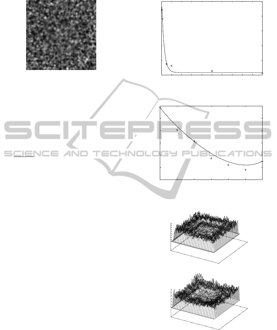
Figure 4: Averaged image with 100 images.

In the evaluations, we generated the successive

images from the original image shown in Fig. 3(a) by

randomly sampling r

( j)

as a Gaussian random vari-

able. By varying the number of the images used for

averaging and the deviation of r

( j)

, the depth recov-

ery error was evaluated. Figure 4 shows the averaged

image f

ave

(x) with 100 images. The value of P by

which the local region size for estimating V[v] is de-

ﬁned is adjusted according to the maximum value of

the theoretical V[v] evaluated by Eq. 5, i.e. P is set as

P =

maxV[v] ×6. The evaluated characteristics of

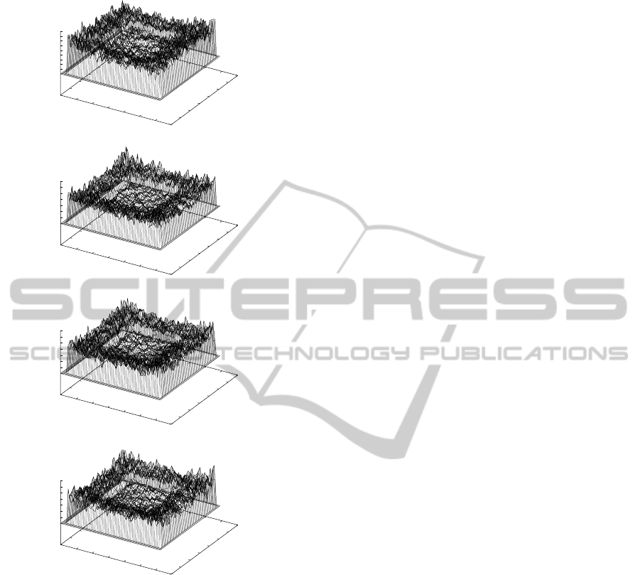
the recovery error are shown in Figs. 5 and 6. Exam-

ples of the depth recovery results are shown in Figs. 7

and 8. In these evaluations, Eqs. 16 with the weights

deﬁned by Eqs. 18, 19 and 20 are employed. These

weights are deﬁned using the true values of V

, which

can not be known in the actual situation, hence we use

the estimated values computed by Eqs. 10, 11 and 12

instead of the true values. Note that Eq. 17 is very

poor for a good recovery in this study.

From Figs. 7 and 8, we can conﬁrm that the outline

of the recovered depth resembles the theoretical one,

but there are a lot of noisy patterns. By increasing

the number of images summed up, the depth recovery

error becomes small, and hence, the noisy patterns in

the estimated V[v] become small a little. On the other

hand, when the motion size is too large, the recovery

error can not become smaller. This means that us-

ing the large motion, the discontinuous regions of the

shape may be recovered as the hardly smooth one.

5 CONCLUSIONS

In this study, we propose a new scheme to recover

a depth map using the camera model imitating ﬁxa-

tional eye movements, especially tremor component.

Our scheme is based on the integral form and the im-

age blurring is mainly used to recover depth, although

we have proposed some differential-formed methods.

We explained the theoretical principle of our scheme

and proposed the simple method to estimate image

1.25

1.3

1.35

1.4

1.45

1.5

0 1000 2000 3000 4000 5000 6000 7000 8000 9000 10000

RMSEs

Frames

Figure 5: Characteristics of depth recovery error with re-

spect to the number of images.

1.2

1.4

1.6

1.8

2.2

2.4

0.001 0.002 0.003 0.004 0.005 0.006 0.007

RMSEs

Deviation of r vector

Figure 6: Characteristics of depth recovery error with re-

spect to the deviation of r

( j)

(a)

0.5

1.5

2.5

3.5

4.5

(b)

0.5

1.5

2.5

Figure 7: Depth recovery results obtained by varying σ

with M = 100: (a) σ

= 0.001 and P = 3; (b) σ

= 0.003

and P = 5.

blurring using the original image and the averaged

image. In this method, by simplifying the problem,

we ignore the constraints for the blurring of this prob-

DEPTH PERCEPTION MODEL EXPLOITING BLURRING CAUSED BY RANDOM SMALL CAMERA MOTIONS

333

(a)

0.5

1.5

2.5

3.5

4.5

(b)

(c)

(d)

Figure 8: Depth recovery results obtained by varying the

number of images with σ

= 0.005 [rad./frame] and P = 9:

(a) M = 100; (b) M = 500; (c) M = 1000; (d) M = 10000.

lem, which should be used to recover accurate depth

map, and hence, we tried to conﬁrm only the feasi-

bility of the proposed integral-formed scheme. From

the results of the numerical evaluations using artiﬁ-

cial images, we can know that the proposed scheme

can get the depth information. In future, we have to

construct the optimal detection method of image blur-

ring caused by the ﬁxational eye movements.

REFERENCES

Bruhn, A. and Weickert, J. (2005). Locas/kanade meets

horn/schunk: combining local and global optic ﬂow

methods. Int. J. Comput. Vision, 61(3):211–231.

Gammaitoni, L., Hanggi, P., Jung, P., and Marchesoni, F.

(1998). Stochastic resonance. Rev. Modern Physics,

70(1):223–252.

Greenwood, P., Ward, L., and Wefelmeyer, W. (1999). Sta-

tistical analysis of stochastic resonance in a simple

setting. Physical Rev. E, 60:4687–4696.

Hongler, M.-O., de Meneses, Y. L., Beyeler, A., and Jacot,

J. (2003). The resonant retina: exploiting vibration

noise to optimally detect edges in an image. IEEE

Trans. Pattern Anal. Machine Intell., 25(9):1051–

1062.

Horn, B. K. P. and Schunk, B. (1981). Determining optical

ﬂow. Artif. Intell., 17:185–203.

Jazwinski, A. (1970). Stochastic processes and ﬁltering the-

ory. Academic Press.

Martinez-Conde, S., Macknik, S. L., and Hubel, D. (2004).

The role of ﬁxational eye movements in visual percep-

tion. Nature Reviews, 5:229–240.

Oliver, C. and Quegan, S. (1998). Understanding synthetic

aperture radar images. Artech House, London.

Propokopowicz, P. and Cooper, P. (1995). The dynamic

retina. Int’l J. Computer Vision., 16:191–204.

Simoncelli, E. P. (1999). Bayesian multi-scale differential

optical ﬂow. In Handbook of Computer Vision and

Applications, pages 397–422. Academic Press.

Stemmler, M. (1996). A single spike sufﬁces: the simplest

form of stochastic resonance in model neuron. Net-

work: Computations in Neural Systems, 61(7):687–

716.

Tagawa, N. (2010). Depth perception model based on ﬁx-

ational eye movements using byesian statistical infer-

ence. In proc. ICPR2010, pages 1662–1665.

Tagawa, N. and Alexandrova, T. (2010). Computational

model of depth perception based on ﬁxational eye

movements. In proc. VISAPP2010, pages 328–333.

VISAPP 2012 - International Conference on Computer Vision Theory and Applications

334