
BAYESIAN PERSPECTIVE-PLANE (BPP) FOR LOCALIZATION
Zhaozheng Hu
1, 2
and Takashi Matsuyama
1
1
Graduate School of Informatics, Kyoto University, Sakyo-Ku, Kyoto, Japan
2
College of Information Science and Technology, Dalian Maritime University, Dalian, China
Keywords: Vision-based Localization, Bayesian Perspective-plane (BPP), Plane Normal, Maximum Likelihood.
Abstract: The "perspective-plane" problem proposed in this paper is similar to the "perspective-n-point (PnP)" or
"perspective-n-line (PnL)" problems, yet with broader applications and potentials, since planar scenes are
more widely available than control points or lines in practice. We address this problem in the Bayesian
framework and propose the "Bayesian perspective-plane (BPP)" algorithm, which can deal with more
generalized constraints rather than type-specific ones to determine the plane for localization. Computation
of the plane normal is formulated as a maximum likelihood problem, and is solved by using the Maximum
Likelihood Searching Model (MLS-M). Two searching modes of 2D and 1D are presented. With the
computed normal, the plane distance and the position of the object or camera can be computed readily. The
BPP algorithm has been tested with real image data by using different types of scene constraints. The 2D
and 1D searching modes were illustrated for plane normal computation. The results demonstrate that the
algorithm is accurate and generalized for object localization.
1 INTRODUCTION
Vision-based localization has many applications in
computer vision, robotics, augmented reality (AR),
simultaneous localization and mapping (SLAM),
and photogrammetric communities (Hartley &
Zisserman, 2004; Desouza et al., 2002; Durrant-
Whyte & Bailey, 2006; Cham et al., 2010). The
basic objective is to compute the position of the
object or the camera in a reference coordinate
system by using either multiple (two or more) or
single image(s). For example, stereo vision is a
commonly used approach for localization from two
images, which can retrieve the 3D coordinates or
position of an object in the scene from image
disparity, baseline width, and camera focal length
(Hartley & Zisserman, 2004). Localization from
single view usually relies on "prior knowledge" of
the scene. In the literatures, many localization
algorithms were developed by utilizing specific
scene constraints, such as well-defined landmarks,
natural or artificial objects, and the abstract points or
lines, etc. For example, landmarks are commonly
used for localization (Adan, 2010). Face position can
be computed by referring to a 3D face model (Sun et
al., 2008). Single image of a window in the street is
possible to localize the camera (Johansson &
Cipolla, 2002). Camera pose can also be computed
from corner structure (Shi et al., 2004). Besides
these particular objects, many researches investigate
the localization problem from a set of abstract points
or lines, namely known as the perspective-n-point
(PnP) and perspective-n-line (PnL) problems (Wolfe
et al., 1991; Kneip et al., 2011; Hu & Matsuyama,
2011). Besides points and lines, the position can also
be computed from a plane or planar object. Planar
structure, i.e., the plane normal and distance, can be
computed from parallel lines, homography, conics,
control points, textures, etc. For example, Hu et al
determine the support plane from the geometric
constraints of three control points (Hu &
Matsuyama, 2011). With four or more planar points,
we can compute the homography and determine the
plane position by decomposition (Zhang, 2000). The
plane normal is also computed from vanishing line,
if two sets of parallel lines are available in the scene
(Lee et al., 2009). Other methods to compute the
plane by using conics, reference lengths, textures,
etc., are also reported in (Hartley & Zisserman,
2004; Guo & Chellappa, 2010; Witkin, 1981).
Existing methods for localization and planar
structure computation from single view are mostly
based on specific scene constraints. These methods
are not generalized or practical enough. On the one
hand, some strict constraints, which are required by
the type-specific algorithm, are not available in the
241
Hu Z. and Matsuyama T..
BAYESIAN PERSPECTIVE-PLANE (BPP) FOR LOCALIZATION.
DOI: 10.5220/0003818902410246
In Proceedings of the International Conference on Computer Vision Theory and Applications (VISAPP-2012), pages 241-246
ISBN: 978-989-8565-04-4
Copyright
c
2012 SCITEPRESS (Science and Technology Publications, Lda.)

scene. On the other hand, some constraints, which
are present in the scene, are difficulty to be utilized
by the type-specific algorithm. In this paper, we
propose the "perspective-plane" problem and
address it by the Bayesian perspective-plane (BPP)
algorithm. The proposed algorithm can utilize more
generalized planar and out-of-plane constraints to
determine the plane for localization.
2 FORMULATION OF
GEOMETRIC CONSTRAINTS
From projective geometry, a physical plane and its
image are related by a 3×3 homography matrix H as
follows (Hartley & Zisserman, 2004; Zhang, 2000)
xHX
1−
≅
(1)
where
≅
means equal up to a scale, x and X are the
coordinates for the image and physical point,
respectively. The homography is computed from the
plane normal and distance according to stratified
reconstruction theories (Hartley & Zisserman, 2004).
With the recovered 2D coordinates, more planar
geometric attributes, such as coordinate, distance,
angle, length ratio, curvature, shape area, etc., are
calculated readily. A metric reconstruction of the
plane is also feasible with known plane normal and
unknown distance. However, the absolute geometric
attributes, such as coordinates, distance, etc., are
equal to the actual ones up to a common scale. And
non-absolute geometric attributes, such as length
ratio, angle, etc., are equal to the actual ones.
Some out-of-plane geometric attributes can also
be computed with a reference plane. For example, an
orthogonal plane can be measured by referring to a
known plane (Wang et al., 2005). If the vanishing
line of a reference plane and one vanishing point
along a reference direction are known, object height,
distance, length ratio, angle, and shape area on the
parallel planes etc., are readily computed (Criminisi
et al., 2000). From projective geometry, both the
vanishing line and the vanishing point along the
normal are computed from the plane normal and the
calibration matrix. Also, if the plane distance is
unknown, those absolute out-of-plane geometric
attributes are computed up to a common scale, while
the non-absolute ones are equal to the actual ones.
Hence, we use
()
NQ
i
to denote the i
th
geometric
attribute, computed from the plane normal N. Scene
prior knowledge can be formulated into constraints
on plane normal. Let
i
u
be the deterministic value
of the geometric attribute that we know a prior. The
measurement error is defined as
(
)
(
)
iii
uNQNd
−
=
(2)
By forcing zero measurement error, we can derive
one geometric constraint on the plane normal
(
)
(
)
0: =−
=
iiii
uNQNdC
(3)
Eq. (3) holds for both planar and out-of-plane
constraints. Planar constraints are derived from prior
knowledge of planar features, while the out-of-plane
constraints are from the out-of-plane ones. The
planar features are those that lie on the plane, such
as the point, line, angle, curve, shape, etc., while the
other are defined as out-of-plane features, such as an
orthogonal line, an angle on another plane, etc. In a
similar way, we can derive a set of geometric
constraints as follow
(
)
(
)
{
}( )
MiuNQNdCC
iiii
,,2,10| "=
=
−
=
=
(4)
3 BAYESIAN
PERSPECTIVE-PLANE (BPP)
3.1 Localization from a Known Plane
An arbitrary planar point can be localized from a
known plane as follows
⎪
⎩
⎪
⎨
⎧
=
=
−
dXN
xKX
T
1
λ
(5)
The first equation in Eq. (5) defines the back-
projection ray, where the 3D point X lies (Hartley &
Zisserman, 2004). It can be determined from the
camera calibration matrix and the image point. The
second one is the plane equation with the normal N
and distance d. If we use the plane to expand a
reference coordinate system, the camera can be
localized as well (Zhang, 2000).
3.2 Plane Normal from MLS-M
3.2.1 Maximum Likelihood Formulation
The plane normal is assumed uniform distribution if
there are no geometric constraint. The distribution
changes from uniform to non-uniform, given one
constrain. Distribution from a set of constraints is
expected to have a dominant peak, from which the
plane normal is solved. Therefore, computation of
the plane normal N is formulated as to maximize the
following conditional probability
VISAPP 2012 - International Conference on Computer Vision Theory and Applications
242

()
M
N
CCCNP ,,,|maxarg
21
"
(6)
By using Bayes’ rule, Eq. (6) is transformed as
()
()()
()
M
M
M
CCCP
NPNCCCP
CCCNP
,,,
|,,,
,,,|
21
21
21
"
"
" =
(7)
Assume that all the constraints are conditionally
independent to each other so that we can derive
()()
∏
=
=
M
i
iM
NCPNCCCP
1
21
||,,, "
(8)
Assume uniform distribution of plane normal and
we can substitute Eq. (8) into Eq. (7) to derive
()()
∏
=
∝
M
i
iM
NCPCCCNP
1
21
|,,,| "
(9)
In order to solve Eq. (6), we need to model
()
NCP
i
|
, which is defined as the likelihood that the
i
th
constraint is satisfied, given the plane normal N.
We set the following rules to develop the model: 1)
the likelihood is determined by the measurement
error. More absolute measurement error yields lower
likelihood. The maximum likelihood is reached if
the measurement error is zero; 2) the maximum
likelihoods (for zero measurement errors) for
different constraints should be equal so that all
constraints contribute equally; 3) the measurement
error should be normalized to deal with the
geometric attributes in different forms, units, and
scales, etc. To meet these requirements, the
normalized Gaussian function was proposed to
model the likelihood as follows
()()
(
)
⎟
⎟
⎠
⎞
⎜
⎜
⎝
⎛
−=
22
2
2
exp
2
1
,|
ii
i
i
iii
u
Nd
uNdG
σ
σπ
σ
(10)
The measurement error is normalized by
i
u
from
Eq. (3). Obviously, Eq. (10) satisfies the first rule.
The likelihood also decreases with the absolute
measurement errors. The maximum likelihood is
reached at zero measurement error. In order to
satisfy the second rule, the standard deviations for
all Gaussian models should be equal:
σ
σ
σ
=
=
ji
.
Hence, the likelihood model is derived as
() ()()
()
⎟
⎟
⎠
⎞
⎜
⎜
⎝
⎛
−==
22
2
2
exp
2
1
|
σ
σπ
i
i
ii
u
Nd
NdGNCP
(11)
Substitution Eq. (11) into Eq. (9) yields
()
(
)
∏
=
⎟
⎟
⎠
⎞
⎜
⎜
⎝
⎛
−∝
M
i
i
i
M
u
Nd
CCCNP
1
22
2
21
2
exp,,,|
σ
"
(12)
The plane normal is thus computed as
(
)
⎟
⎟
⎠
⎞
⎜
⎜
⎝
⎛
−
∑
=
M
i
i
i
N
u
Nd
1
22
2
2
expmaxarg
σ
(13)
3.2.2 Searching for Maximum Likelihood
A maximum likelihood searching model (MLS-M)
is used to solve Eq. (13). Two searching modes of
2D and 1D are proposed in the following.
a. 2D searching mode
A unit normal corresponds to a point on the
Gaussian sphere surface so that the searching space
is defined. In practice, we search on the Gaussian
hemisphere to reduce the searching space into half,
because only the planes in front of the camera are
visible in the image. A uniform sampling is realized
by evenly partition Gaussian hemisphere, which can
be solved by using the recursive zonal equal area
sphere partitioning algorithm (Leopardi, 2004). The
likelihood for each sample is computed so that the
maximum likelihood is calculated by sorting, the
corresponding plane normal is then determined.
Since Gaussian sphere in 3D space is 2D, we call it a
2D searching mode.
b. 1D searching mode
1D searching mode is feasible if one linear
constraint is available in the scene. In practice, some
linear constraints can be derived from parallel lines,
orthogonal lines or planes, etc. We introduced the
1D searching mode by using orthogonal line as an
example. Let
L
be the orthogonal line, with the
image
l
. Because
L
is parallel to the plane normal,
the vanishing point
N
V
along the normal lies on
l
and satisfy the following equation
()
(
)
0=== NlKKNlVl
T
TT
N
T
(14)
The normal N also lies on Gaussian sphere so that
(
)
⎪
⎩
⎪
⎨
⎧
=
=
1
0
NN
NlK
T
T
T
(15)
Eq. (15) defines a circle in 3D space, which is the
intersection of the plane with the Gaussian sphere.
Therefore, we need to search on the circle (actually
half of the circle). Similarly, a uniform sampling on
the circle is required. The likelihood for each sample
is computed. And the maximum likelihood is finally
searched to solve the plane normal.
3.3 Plane Distance Computation and
Localization
Assume unit plane distance and re-write Eq. (5) as
BAYESIAN PERSPECTIVE-PLANE (BPP) FOR LOCALIZATION
243
⎪
⎩
⎪
⎨
⎧
=
′
′
=
′
−
1
1
XN
xKX
T
λ
(16)
Compared to Eq. (5), it can be derived that
XX
≅
′
.
Hence, we can localize all the planar points in the
camera coordinate system up to a common scale. In
order to compute the actual coordinates, a reference
length or distance is required. For example, the scale
can be determined from the actual length
AB
L
between two points A and B as follows
BA
AB
XX
L
′
−
′
=
β
(17)
where
A
X
′
and
B
X
′
are the 3D coordinates of two
points that are computed from Eq. (16). With the
computed scale factor, the actual plane distance is
β
=d
. And the actual 3D position is
XX
′
=
β
(18)
4 EXPERIMENTAL RESULTS
The proposed algorithm was tested with two real
image experiments. A Nikon D700 camera was used
to generate the real images of 2218
×1416 (pixel)
resolution. It was calibrated with Zhang's calibration
algorithm (Zhang, 2000) with 1369.2-pixel focal
length and principle point at [1079, 720]
T
(pixel).
The calibration results were used for planar structure
computation and localization. As there are various
scene constraints in practice, it is difficult to discuss
all of them. We chose two representative constraint
types of known angle and length ratios to validate
the proposed model in the experiments.
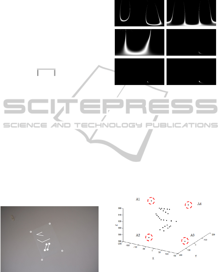
Figure 1: Three planar constrains (two known angles and
one length ratio) from lines and points for localization.
The algorithm was tested with planar constraints
first. Figure 1 shows an image of a white paper
attached on the wall. Six line segments were drawn
Figure 2: From upper left to lower right: (a) (b) (c)
likelihoods from three geometric constraints, (d) the joint
likelihood, (e) positions of the 30 normal of the highest
likelihoods; (f) the computed normal marked by ‘+’.
on the paper. We derived two angles (34.1 and 126.6
degrees) from L1-L2 and L3-L4, and one length
ratio between the distances of M1-M2 and M3-M4
to derive three planar constraints. The 2D searching
mode was applied then. The likelihoods from
different geometric constraints are shown in Figure
2(a)~(c), where the non-uniform distributions of the
plane normal are observed. The joint likelihood is
shown in Figure 2(d), where a bright area on the
bottom is observed. Figure 2(e) shows the 30 plane
normal with the highest likelihoods. The plane
normal computed from the joint likelihood map is
marked by '+' (see Figure 2(f)), with the result
[0.0993 0.1679 0.9808]
T
.
Figure 3: Localize points and lines in the camera
coordinate system (unit in mm).
The plane distance was computed by using the
reference length of the white paper (297mm). The
points on the plane were localized. Figure 3 shows
3D positions of the points on the six line segments,
and the four corners (A1~A4 marked by 'o'), all in
L1
L2
L3
L4
M1
M2
M3
M4
A4
A2
A3
A1
VISAPP 2012 - International Conference on Computer Vision Theory and Applications
244
the camera coordinate system. The computation
results were validated as follow. The lengths of A2-
A3, A3-A4, and A1-A4 were computed from the
recovered 3D coordinates as 206.7, 294.6, and 211.8
(mm), respectively. Compared to ground truth data
(the size of the white paper), the absolute errors are
3.3, 2.4, and 1.8 (mm), corresponding to 1.6%,
0.8%, and 0.9% relative errors. It demonstrates that
the proposed model is accurate.
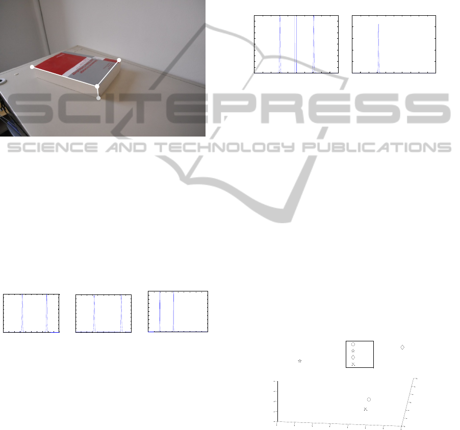
Figure 4: Localization from 3D corner constraints.
The algorithm was further tested with both planar
and out-of-plane constraints by using 1D searching
mode. As shown in Figure 4, a 3D corner structure
of a book is defined by the three orthogonal lines of
L1, L2, and L3. From these three lines, three planes
are defined as L1-L2, L1-L3, L2-L3. For each plane,
we derived two constraints: 1) one orthogonal line to
the plane; 2) one right angle between the other two
lines on the plane, as shown in Figure 4. They were
used to localize each plane.
Figure 5: From left to right: likelihoods of the normal of
the planes defined by: a) L1-L2, b) L1-L3, c) L2-L3.
The 1D searching mode was applied. The
searching circles were defined from the orthogonal
line constraints, on which 10,000 points were
uniformly sampled, respectively. The likelihoods for
each normal of the three planes were computed
afterwards (see Figure 5(a)~(c)). For each plane, two
peaks are observed from the likelihood curve, which
indicates two solutions (also see multiple solutions
in (Shi et al., 2004)). Hence, eight combinations for
the normal of the three planes are derived, two of
which satisfy the mutually orthogonality constraints.
In order to eliminate the ambiguity, we utilized one
more constraint from the ratio of the length (M0-
M1) to the width (M0-M2) to uniquely determine
the normal of the plane L1-L2. The likelihood from
such constraint and the joint likelihood are
illustrated in Figure 6. In the joint likelihood, a
unique peak is observed (see Figure 6(b)). From the
joint likelihood, the maximum likelihood was
searched and the normal to the L1-L2 plane was
computed as [-0.0022 0.8425 0.5387]
T
. With the
computed L1-L2 normal, the normal for the other
two planes were also uniquely determined.
Figure 6: From left to right: a) likelihood from the length
ratio constraint; b) joint likelihood from all constraints.
We used one actual length to compute the plane
distance and localize the corner points in the camera
coordinate system. Their 3D positions are shown in
Figure 7. The camera was also localized in the
reference coordinate system, defined by the corner
structure, with M0 as the origin, and L1, L2, L3 as
the three axes, where the camera position is [-21.64,
-23.82, -12.26]
T
(in cm). Hence, the object and the
camera were localized from each other. We
validated the results as follows. The calculated 3D
coordinates were used to fit the three lines. The lines
are mutually orthogonal and have an angle of 90
degrees in between, which are used as ground truth.
The computed angles in-between are 89.4, 88.1, and
94.1 degrees, respectively, with the absolute errors
of 0.6, 1.9, and 4.1 degrees. The relative errors are
0.7%, 2.1%, and 4.6%, with the average 2.4%. The
results demonstrate that the algorithm is accurate.
Figure 7: Localize the four corner points in the camera
coordinate system (unit in cm)
5 CONCLUSIONS
In this paper, we proposed the Bayesian perspective-
0 1000 2000 3000 4000 5000 6000 7000 8000 9000 10000
0
0.1
0.2
0.3
0.4
0.5
0.6
0.7
0.8
0.9
1
Number of sampled normal
The relative probability
0 1000 2000 3000 4000 5000 6000 7000 8000 9000 10000
0
0.1
0.2
0.3
0.4
0.5
0.6
0.7
0.8
0.9
1
Number of sampled normal
The relative probability
0 1000 2000 3000 4000 5000 6000 7000 8000 9000 10000
0
0.1
0.2
0.3
0.4
0.5
0.6
0.7
0.8
0.9
1
Number of sampled normal
The relative probability
0 1000 2000 3000 4000 5000 6000 7000 8000 9000 10000
0
0.1
0.2
0.3
0.4
0.5
0.6
0.7
0.8
0.9
1
Number of sampled normal
The relative probability
0 1000 2000 3000 4000 50 00 6000 700 0 8000 9000 10 000
0
0.5
1
1.5
2
2.5
x 10
-6
Number of sampled normal
The relative probability
-25
-20
-15
-10
-5
0
5
10
-4
-2
0
2
4
6
8
30
35
40
45
50
Z
Y
X
M0
M1
M2
M3
L1
L2
L3
M0
M3
M1
M2
BAYESIAN PERSPECTIVE-PLANE (BPP) FOR LOCALIZATION
245

plane (BPP) algorithm to address the "perspective-
plane" problem, which can localize object/camera by
determining planar structure from more generalized
planar and out-of-plane constraints. Computation of
the plane normal is formulated as a maximum
likelihood problem and is solved by MLS-M. Both
2D and 1D searching modes were presented. The
BPP algorithm has been tested with real image data.
The results show that the proposed algorithm is
generalized to utilize different types of constraints
for accurate localization.
ACKNOWLEDGEMENTS
The work presented in this paper was sponsored by a
research grant from the Grant-In-Aid Scientific
Research Project (No. P10049) of the Japan Society
for the Promotion of Science (JSPS), Japan, and a
research grant (No. L2010060) from the Department
of Education (DOE), Liaoning Province, China.
REFERENCES
Hartley, R., and Zisserman, A., 2004. Multiple view
geometry in computer vision, Cambridge, Cambridge
University Press, 2
nd
Edition.
Desouza, G. N., and Kak, A. C., 2002. Vision for mobile
robot navigation: a survey, IEEE Trans on Pattern
Analysis and Machine Intelligence, 24(2): 237-267.
Durrant-Whyte, H. and Bailey, T., 2006. Simultaneous
Localization and Mapping (SLAM): part I the
essential algorithms, IEEE Robotics and Automation
Magazine, 13 (2): 99-110.
Cham, T., Arridhana, C., Tan, W. C., Pham, M. T., Chia,
L. T., 2010. Estimating camera pose from a single
urban ground-view omni-directional image and a 2D
building outline map, IEEE International Conference
on Computer Vision and Pattern Recognition (CVPR),
IEEE Press.
Adan, A., Martin, T., Valero, E., Merchan, P., 2009.
Landmark real-time recognition and positioning for
pedestrian navigation, CIARP, Guadalajara, Mexico,
Sun, Y., and Yin, L., 2008. Automatic pose estimation of
3D facial models, IEEE International Conference on
Pattern Recognition (ICPR), IEEE Press.
Johansson, B., and Cipolla, R., 2002. A system for
automatic pose-estimation from a single image in a
city scene, In IASTED Int. Conf. Signal Processing,
Pattern Recognition and Applications, Crete, Greece
Shi, F., Zhang, X., and Liu, Y., 2004. A new method of
camera pose estimation using 2D-3D corner
correspondence, Pattern Recognition Letters, 25(10):
805-809.
Wolfe, W., Mathis, D., Sklair, C., and Magee, M., 1991.
The perspective view of three Points, IEEE
Transaction on Pattern Analysis and Machine
Intelligence, 13(1): 66-73.
Kneip, L., Scaramuzza, D., and Siegwart, R., 2011. A
novel parameterization of the perspective-three-point
problem for a direct computation of absolute camera
position and orientation, IEEE International
Conference on Computer Vision and Pattern
Recognition (CVPR), IEEE Press.
Hu, Z., and Matsuyama, T., 2011. Perspective-three-point
(P3P) by determining the support plane, International
Conference on Computer Vision Theory and
Applications (VISAPP), SciTePress.
Zhang, Z., 2000. A flexible new technique for camera
calibration, IEEE Transactions on Pattern Analysis
and Machine Intelligence, 22(11):1330-1334.
Lee, D. C., Hebert, M., and Kanade, T., 2009. Geometric
reasoning for single image structure recovery, IEEE
International Conference on Computer Vision and
Pattern Recognition (CVPR), IEEE Press.
Guo, F., and Chellappa, R., 2010. Video metrology using a
single camera, IEEE Trans on Pattern Analysis and
Machine Intelligence, 32(7): 1329 -1335.
Witkin, A. P., 1981. Recovering surface shape and
orientation from texture, Artificial Intelligence,
17(1-3): 17-45.
Wang, G., Hu, Z., Wu, F., and Tsui, H., 2005. Single view
metrology from scene constraints,
Image and Vision
Computing, 23(9): 831-840.
Criminisi, A., Reid, I., and Zisserman, A., 2000. Single
view metrology, International Journal of Computer
Vision, 40(2): 123-148.
Leopardi, P., 2006. A partition of the unit sphere into
regions of equal area and small diameter, Electronic
Transactions on Numerical Analysis, 25(12):309-327.
VISAPP 2012 - International Conference on Computer Vision Theory and Applications
246
