
SELF-CONSISTENT 3D SURFACE RECONSTRUCTION AND
REFLECTANCE MODEL ESTIMATION OF METALLIC SURFACES
Steffen Herbort and Christian W
¨
ohler
Image Analysis Group, TU Dortmund, Otto-Hahn-Straße 4, 44227 Dortmund, Germany
Keywords:
3D Surface Reconstruction, Active Range Scanning, Image-based 3D Reconstruction, Data Fusion, Re-
flectance Model Estimation.
Abstract:
3D surface reconstruction data measured with active range scanners typically suffer from high-frequency noise
on small scales. This poses a problem for highly demanding surface inspection tasks and all other applications
that require a high accuracy of the depth data. One way to achieve increased 3D reconstruction accuracy is
the fusion of active range scanning data and photometric image information. Typically, this requires modeling
of the surface reflectance behavior, which, in turn, implies the surface to be known with high accuracy to
determine valid reflectance parameters as long as no calibration object is available. In this study, we propose
an approach that provides a detailed 3D surface reconstruction along with simultaneously estimated param-
eters of the reflectance model. For 3D surface reconstruction, we employ an algorithm that combines active
range scanning data for large-scale accuracy with image-based information for small-scale accuracy. For in-
ferring the reflectance function, we incorporate the estimation of the reflectance model into a self-consistent
computational scheme that successively increases the resolution and thus determines the reflectance parame-
ters based on refined depth information. We present results for a homogeneous dark rough metallic surface,
which is reconstructed based on a single coarse 3D scan and 12 images acquired under different illumination
conditions.
1 INTRODUCTION
Active range scanning approaches typically suffer
from high-frequency noise and thus lack the capa-
bility to perceive and resolve fine surface details es-
pecially for non-diffusely reflecting surfaces. While
filtering may reduce high-frequency noise and re-
cover some of the the underlying details, the over-
all quality and accuracy is not improved significantly
while the effective lateral resolution decreases. If
one wants to truly enhance the amount of surface de-
tail, it is desirable to supplement the absolute depth
data obtained by active range scanners with gradient
information obtained using image-based approaches
like shape from shading (Horn, 1970) or photometric
stereo (Woodham, 1980). The crucial problem lies in
finding an approach that fuses both data sources and at
the same time exploits the mutual advantages: Range
scanning approaches provide robust large-scale data
with high-frequency noise, while image-based data
provide accurate small-scale details but tend to devi-
ate systematically from the true large-scale shape. A
well-known example for that fusion process has been
proposed by Nehab et al. (Nehab et al., 2005) and
their results clearly demonstrate the improved small-
scale accuracy. However, their approach only deals
with pre-existing data and omits the gradient deter-
mination stage, which is challenging e.g. for metal-
lic surfaces. Later approaches for fusing depth data
and photometric image information (cf. e.g. (W
¨
ohler
and d’Angelo, 2009) and references therein) include
an estimation of the surface gradients but still assume
the reflectance function to be known in advance.
It is thus interesting from a theoretical and rele-
vant from a practical point of view to develop a self-
consistent approach that incorporates all steps nec-
essary for 3D surface reconstruction, including an
estimation of the reflectance function. Apart from
surface inspection, the demand for highly accurate
surfaces comes from other fields as well. In com-
puter graphics, the problem of determining the re-
flectance function from arbitrarily shaped surfaces
commonly lacks accuracy due to the fact that the ex-
amined surface shape is not known to the required
level of detail (Weyrich et al., 2008). While sev-
eral image-based methods solve that problem by as-
suming known shapes (Matusik et al., 2003b), this
is only possible for surfaces which provide all illu-
114
Herbort S. and Wöhler C..
SELF-CONSISTENT 3D SURFACE RECONSTRUCTION AND REFLECTANCE MODEL ESTIMATION OF METALLIC SURFACES.
DOI: 10.5220/0003819701140121
In Proceedings of the International Conference on Computer Vision Theory and Applications (VISAPP-2012), pages 114-121
ISBN: 978-989-8565-04-4
Copyright
c
2012 SCITEPRESS (Science and Technology Publications, Lda.)
mination and viewing geometries required for a re-
liable reflectance parameter estimation. Once this
precondition is fulfilled and the surface is known
to the required level of detail, the determination of
the reflectance function becomes a problem of non-
linear model adaptation using methods such as the
Levenberg-Marquardt algorithm (Mor
´
e, 1978). As a
result of previous and current research, a large vari-
ety of reflectance models have been developed, which
are typically selected based on the material at hand.
The most popular ones include the classical Lamber-
tian model (Lambert, 1760; Horn, 1989) for strictly
diffuse surfaces, the Phong model (Phong, 1975) for
empirically modeled specularities, its more physically
motivated version (Lewis, 1994), its generalized ver-
sion (Lafortune et al., 1997), and more specialized
models for metals and rough surfaces (Cook and Tor-
rance, 1981; Beckmann and Spizzichino, 1987) and
anisotropic surfaces (Ward, 1992).
Image-based algorithms analyze the object ap-
pearance and thus commonly depend on a reflectance
model that is known a priori as accurately as possi-
ble. Unfortunately, this usually requires the surface
shape to be known in advance with very high accu-
racy, as discussed above. To overcome that drawback,
we present a self-consistent approach for the simulta-
neous determination of surface shape and reflectance
function parameters for strongly non-Lambertian sur-
faces. In contrast to methods from the field of com-
puter graphics, e.g. (Lensch et al., 2003), we do not
only change local surface normals to model the ap-
pearance of the object in a rendered image, but actu-
ally incorporate that information into the 3D recon-
struction of the surface.
The critical aspect lies in the determination of re-
flectance parameters without fine surface shape data
being available. Our approach thus uses strongly
downsampled absolute depth and image data to de-
termine initial reflectance function parameters. These
are reliable since the absolute depth and image data
are reasonably accurate on that scale. The surface re-
construction algorithm then uses that information and
computes a refined surface. The process then itera-
tively continues on a higher resolution scale (cf. Sec-
tion 2). The alternating scheme of reflectance func-
tion estimation and surface reconstruction thus suc-
cessively refines the 3D surface reconstruction and
the estimated reflectance parameters (cf. Section 3).
For data acquisition, we use a calibrated range scan-
ning system with 12 attached LED light sources with
known (calibrated) illumination directions and a sin-
gle camera position. Our experimental results are de-
scribed in Section 4.
downsample 1:2
K
images
images
images
images depth
BRDF estimation
surface reconstruction
p
K
, q
K
, z
K
upsampling (factor 2)
BRDF
K
K=K - 1
optimized
optimized
K <
0 ?
N
Y
full resolu-
tion result
initial BRDF estimation
median-
filter
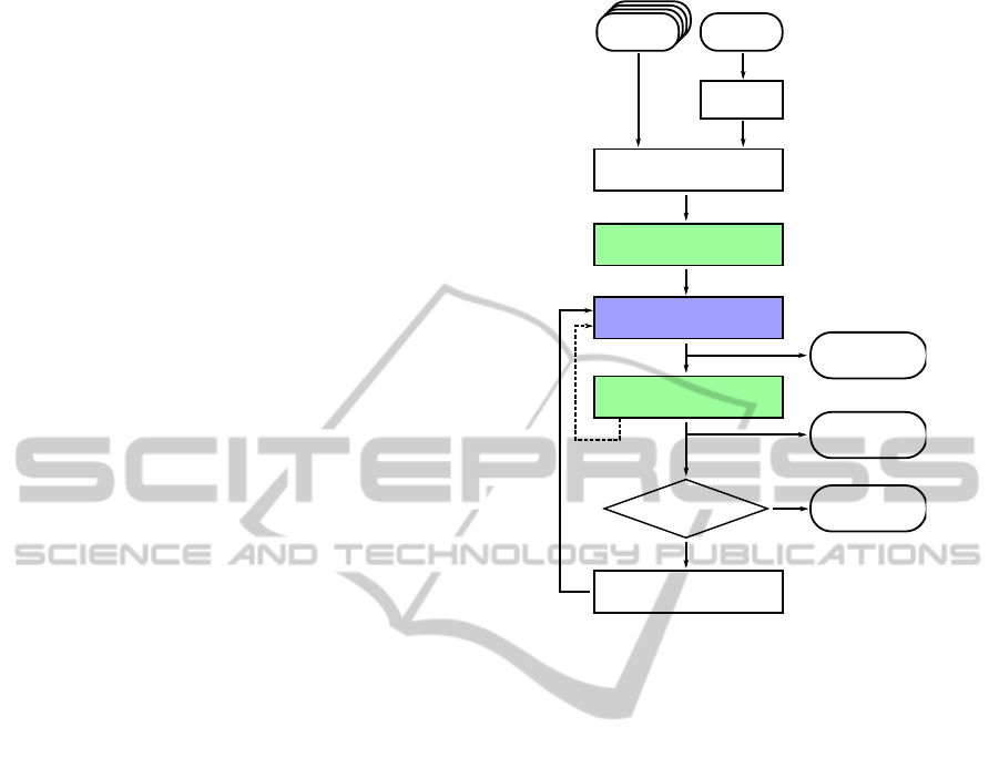
Figure 1: Overview of the self-consistent algorithm for
3D surface reconstruction and reflectance parameter esti-
mation.
2 SELF-CONSISTENT
RECONSTRUCTION
Fig. 1 illustrates the proposed self-consistent 3D re-
construction algorithm. The main elements are the
estimation of the reflectance parameters (green) and
the surface reconstruction (blue). The algorithm starts
with the given image and depth data, which are ini-
tially subsampled by a factor of 2
K
with appropriate
spatial low-pass filtering to avoid aliasing. The sub-
sampling stage ensures the removal of spurious high
spatial frequency components from the range scan-
ner data and thus provides the basis for robust re-
flectance estimation on that scale. Once the initial
reflectance parameters are known, the reconstruction
exploits the reflectance information to incorporate the
image-based depth data. The successive steps “sur-
face reconstruction” and “BRDF estimation” can be
iterated in an inner loop (cf. dashed line in Fig. 1)
without increasing the current resolution scale. Af-
terwards, the result of the 3D reconstruction stage is
upsampled by a factor of 2 using bicubic interpola-
tion and then serves as the initialization for the next
iteration. The algorithm terminates when the full res-
olution scale is reached.
SELF-CONSISTENT 3D SURFACE RECONSTRUCTION AND REFLECTANCE MODEL ESTIMATION OF
METALLIC SURFACES
115

3 SURFACE RECONSTRUCTION
AND BRDF ESTIMATION
In this paper, we will use u ∈ [1...N] and v ∈ [1...M]
to denote the integer pixel coordinates of an image
I ∈ R
N×M
. The image data I contain intensity mea-
surements for each pixel, and the available range
scanner data z
RS
(u,v) provide pixel-synchronous ab-
solute depth measurements for most but generally not
all image pixels, i.e. there may be gaps in the absolute
depth data.
Local illumination directions, viewing directions,
and surface normals are denoted by the vectors
~
s(u,v),
~v(u,v), and ~n(u,v), respectively, with k
~
sk
2
= k~vk
2
=
k~nk
2
= 1. The vector ~r denotes the incident light di-
rection mirrored at the respective surface normal. The
reflectance model parameters P are introduced later
when the applied reflectance model M is discussed.
The reflectance function itself is termed BRF (Bidi-
rectional Reflectance Function) or BRDF (Bidirec-
tional Reflectance Distribution Function).
The algorithm computes the optimized surface
gradient fields
p(u,v) =
∂z(u,v)
∂x
= ∂
x
z(u,v) = z
x
(u,v) (1)
q(u,v) =
∂z(u,v)
∂y
= ∂
y
z(u,v) = z
y
(u,v) (2)
and the optimized surface z
∗
(u,v). A rendered image
of the surface obtained using the reflectance function
of the surface, a set of surface gradients, illumination
and viewing directions is denoted “reflectance map”
R according to
R = R (p(u,v),q(u,v),
~
s(u,v),~v(u,v),~n(u,v),P,M).
(3)
An approach for recovering and fusing absolute depth
z
RS
and gradient data (p,q) has been proposed by us
previously (Herbort et al., 2011). The algorithm is
an extension of Horn’s method for the simultaneous
recovery of height and gradients (Horn, 1989). While
Horn’s approach operates solely on image data, the
extension regards the fusion with absolute depth data.
To give a complete background for the approach
presented in this study and to provide better expla-
nations, we summarize the main ideas and give an
overview of its capabilities: The algorithm as such
minimizes the overall error
E = E
I
+ γ E
int
+ δ E
RS
(4)
according to
z
∗
= argmin
p,q,z
(E
I
+ γ E
int
+ δ E
RS
) (5)
by finding an optimal surface z
∗
(u,v), which is com-
posed of the gradient field (p(u,v),q(u,v)). The
weight parameters γ and δ have to be determined em-
pirically, i.e. by manually choosing a set of parame-
ters that lets the optimization scheme iterate and con-
verge. Each component of the error function E con-
tributes to different aspects that enforce certain re-
strictions upon the optimal surface. The intensity er-
ror
E
I
=
∑
u,v
(I − R)
2
(6)
determines the difference between the observed origi-
nal image I and the reflectance map R. The extension
towards several images is straightforward by evalua-
tion of the mean error over all images and their re-
spective reflectance maps. The error term E
I
causes
the optimized surface to alter its gradients until the
image and the reflectance map match as closely as
possible. The integrability error
E
int
=
∑
u,v
(z
x
− p)
2
+ (z
y
− q)
2
(7)
denotes the deviations of the estimated gradient field
from the gradients of the determined surface, i.e. from
an integrable gradient field, and thus prevents the oc-
currence of local gradient spikes. The range scanner
depth gradient error
E
RS
=
∑
u,v
(∂
x
(G ∗ z
rs
) − G ∗ p)
2
+(∂
y
(G ∗ z
rs
) − G ∗ q)
2
(8)
measures the deviation of the estimated surface gra-
dients from those derived from the range scanner data
on large spatial scales. This is achieved by removing
small surface details by convolution with a (Gaussian)
low-pass filter G, which then allows an adaptation of
the low spatial frequency components of the recon-
structed surface gradients to those of the range scan-
ner data (Herbort et al., 2011).
The generation of the reflectance map R requires
the reflectance properties of the surface to be known.
This is typically achieved in a data driven or model
driven way (Matusik et al., 2003a). In our algorithm,
we apply a reflectance model, since there is only a
limited range of viewing directions available if, as in
our case, a fixed camera is used. The estimation of the
model from sparse data is usually possible and robust,
while the inevitable interpolations of data driven ap-
proaches possibly produce unexpected results. In the
following, the chosen model (cf. Section 1 for other
examples) is discussed.
The three-component Lambert/Phong model (Na-
yar et al., 1990) has been applied to isotropic surfaces
with non off-specular reflectance behavior (W
¨
ohler
and d’Angelo, 2009). The observed intensity is de-
scribed by
I = I
0
ρ [~n ·
~
s + σ
l
(~v ·~r)
m
l
+ σ
s
(~v ·~r)
m
s
]. (9)
VISAPP 2012 - International Conference on Computer Vision Theory and Applications
116

3
1
2
3
Figure 2: Overview of the experimental setup. The object
has a height of about 50 mm, the distance between the ob-
ject and the scanner (1), camera (2), and illumination (3)
amounts to approximately 250 mm.
Its parameters are the intensity I
0
of the incident light,
the surface albedo ρ, the specular lobe strength σ
l
, the
specular lobe width m
l
, the specular spike strength
σ
s
, and the specular spike width m
s
(W
¨
ohler and
d’Angelo, 2009). A more generalized form allows a
directional diffuse behavior according to
I = I
0
ρ [(~n ·
~
s) + σ
ds
(~n ·
~
s)
m
ds
+ σ
l
(~v ·~r)
m
l
+ σ
s
(~v ·~r)
m
s
] (10)
with the directional diffuse width m
ds
and strength
σ
ds
. In our experiments (cf. Section 4), this model
has been shown to be flexible enough to represent the
reflectance behavior, while having a feasible number
of 7 parameters (the term I
0
ρ can be set to the “ef-
fective albedo” ρ
eff
). The directional diffuse term has
empirically proven to have a favorable effect on the
3D reconstruction accuracy when few light sources
(i.e. images) are available. Note that the system de-
scribed in this study poses almost no restrictions re-
garding the applied reflectance model. The only re-
quirements are the capability of the reflectance func-
tion to model the reflectance behavior and the solv-
ability of the fitting problem, i.e. it must be possible
to obtain the reflectance model parameters from the
given/obtained data I, p, q, and z.
4 EXPERIMENTAL RESULTS
This section initially provides an overview of the ex-
perimental setup. The obtained results are then pre-
sented and discussed.
4.1 Experimental Setup
Since our range scanning system
1
already contains
a camera
2
and records pixel-synchronous depth and
image data, there is no need for data registration
prior to the reconstruction. All 12 attached LED
light sources
3
have been calibrated using a white
diffuse sphere
4
and solving Lambert’s law I(u,v) =
I
0
ρ (~n(u,v) ·
~
s) for the global light direction
~
s and
the intensity I
0
. In contrast to the popular method
to use a specularly reflecting sphere, using the Lam-
bertian sphere yields more robust results due to the
larger number of measurements being involved in the
optimization. The obtained phase angles, i.e. the an-
gles between the illumination directions and the view-
ing direction, range from 18
◦
to 67
◦
. Note that the
bright regions in the intensity images exhibit very
strong specular spikes, as they are typical for metal-
lic surfaces. To account for these large dynamic vari-
ations within the image due to the dark surface and
the strong specular spikes of the metallic material, we
recorded high dynamic range (HDR) images.
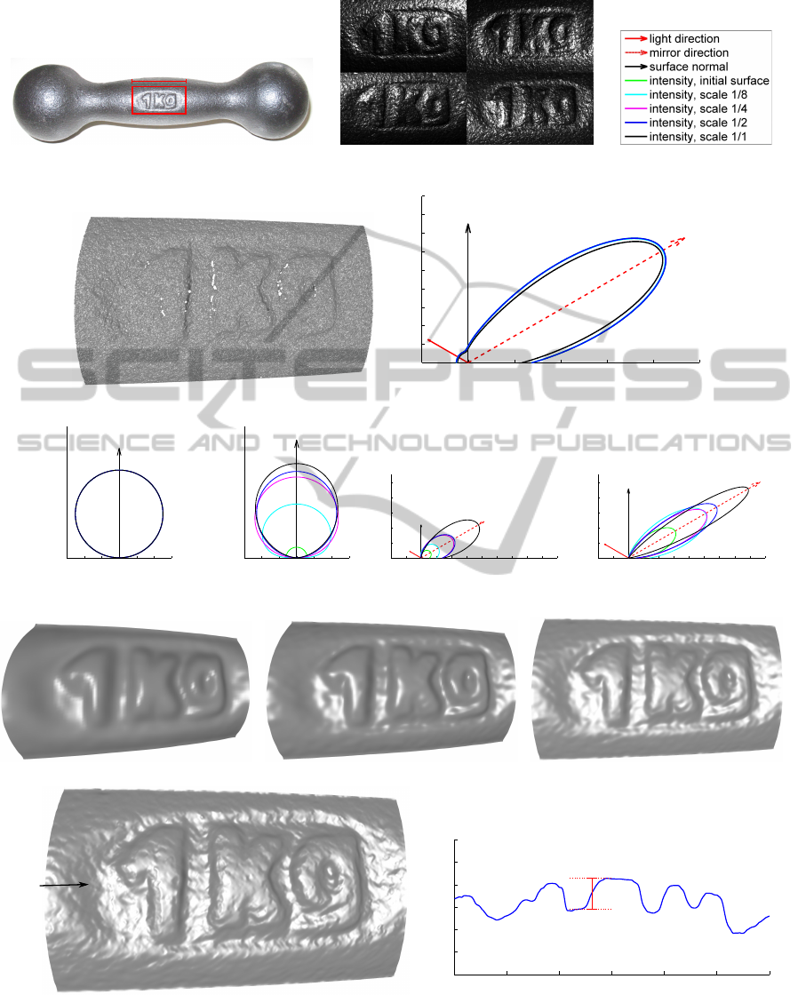
4.2 Results
The results for the 3D reconstruction of an emboss-
ing on the surface of a metallic dumbbell consisting
of dark cast iron are presented in Fig. 3. The object
and the area of interest are depicted in Fig. 3(a), the
input data for the algorithm are shown in Fig. 3(b)
and 3(d). Four of the 12 images acquired under dif-
ferent illumination directions (cf. Fig. 3(b)) and the
raw scanner data (cf. Fig. 3(d)) are shown as well.
Figs. 3(j)–3(m) illustrate how the surface evolves over
4 iterations (K = 3) from a coarse surface at 1/8
of the full scale (cf. Fig. 3(j)) over the intermediate
scales 1/4 (cf. Fig. 3(k)) and 1/2 (cf. Fig. 3(l)) to the
full scale where the resolution of the 3D surface re-
construction reaches the full resolution of the images
(300 × 700 pixels at a scale of 42 µm per pixel) as
shown in Fig. 3(m). Note that with each iteration,
an increasing amount of surface detail becomes vis-
ible and is thus incorporated into the reconstructed
surface. The comparison of the images and the sur-
face shows correspondences between surface bumps
and their bright or dark counterparts in the images.
1
ViALUX zSnapper Vario, structured/modulated light
range scanner
2
AVT pike 421B, 14 Bit monochrome CCD camera,
2048 × 2048 pixels
3
Seoul P4 LED, λ ≈ 525nm (green), luminous flux ap-
proximately 120 lm
4
30 mm diameter, manufactured by Optopolymer, Mu-
nich
SELF-CONSISTENT 3D SURFACE RECONSTRUCTION AND REFLECTANCE MODEL ESTIMATION OF
METALLIC SURFACES
117
≈3cm
(a) Metallic dumbbell, the ROI for the reconstruction is indi-
cated in red.
(b) 4 out of 12 HDR images, 400×700 pixels, lateral
resolution 0.042mm per pixel.
(c) Legend for reflectance func-
tion plots.
(d) Raw range scanner data.
−50 0 50 100 150 200 250
0
20
40
60
80
100
120
140
160
180
observed intensity (x component)
observed intensity (y component)
(e) Development of the full reflectance function.
−0.4 −0.2 0 0.2 0.4 0.6
0
0.5
1
1.5
observed intensity (x component)
observed intensity (y component)
(f) Diffuse component 1.
−0.4 −0.2 0 0.2 0.4 0.6
0
0.5
1
1.5
observed intensity (x component)
observed intensity (y component)
(g) Diffuse component 2.
−4 −2 0 2 4 6 8 10 12 14 16 18
0
2
4
6
8
10
observed intensity (x component)
observed intensity (y component)
(h) Specular lobe.
−4 −2 0 2 4 6 8 10 12 14 16 18
0
2
4
6
8
10
observed intensity (x component)
observed intensity (y component)
(i) Specular spike.
(j) Reconstruction result at scale 1/8. (k) reconstruction result at scale 1/4. (l) reconstruction result at scale 1/2.
depth profile,
see Fig. (n)
(m) reconstruction result at full scale (400 ×700 pixels.)
0 5 10 15 20 25 30
−1
−0.5
0
0.5
1
1.5
2
x [mm]
z [mm]
0.69mm
(n) Depth difference measurement on a cross-sectional surface profile
(cf. arrow in (m)).
Figure 3: Experimental results for an embossing in a metallic dumbbell consisting of dark cast iron. In (f)–(i), the diffuse
components are plotted with the direction
~
s of incident light varying over the upper hemisphere, while the specular components
are plotted with the viewing direction~v being varied.
VISAPP 2012 - International Conference on Computer Vision Theory and Applications
118
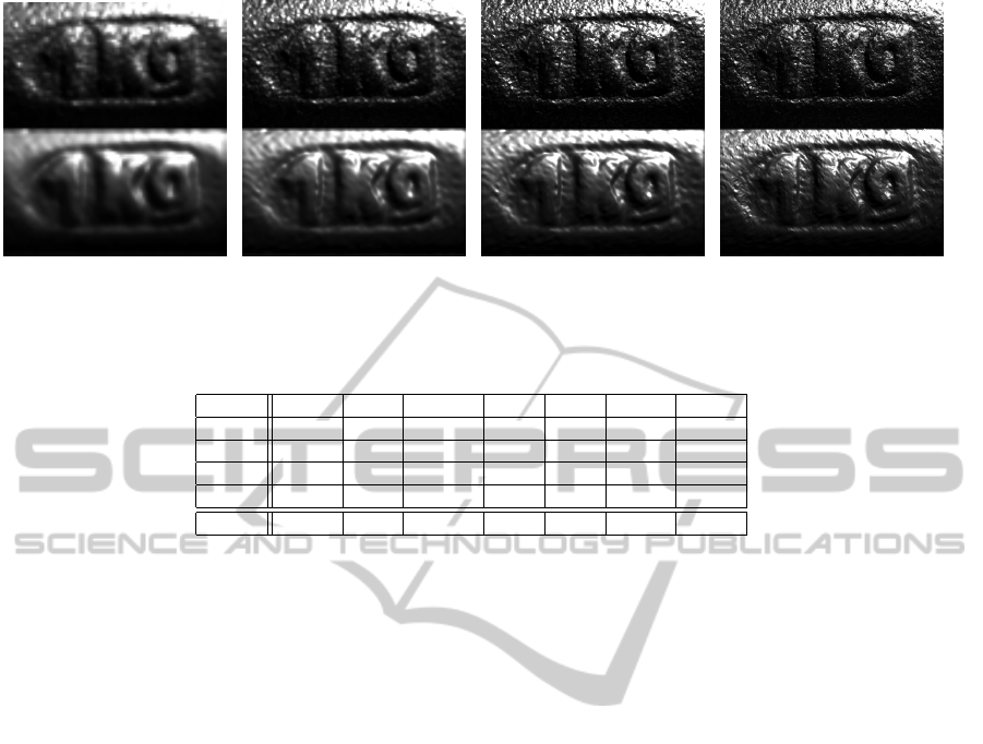
(a) Scale 1/8SSIM = 0.85962 (b) Scale 1/4SSIM = 0.84261 (c) Scale 1/2SSIM = 0.88546 (d) Scale 1/1SSIM = 0.92896
Figure 4: Details regarding the final reflectance maps for different scales under illumination from one selected LED. For each
image, the upper half shows the image data and the lower half the reflectance map.
Table 1: Determined reflectance function parameters for each reconstruction scale and the final result.
scale ρ
eff
σ
ds
m
ds
σ
l
m
l
σ
s
m
s
initial 17.24 0.12 0.0001 1.46 1.85 7.10 9.21
1/8 10.52 0.61 0.45 2.62 1.79 11.75 9.88
1/4 11.59 0.92 0.91 4.83 3.65 11.83 15.03
1/2 12.42 0.98 1.24 5.01 4.05 13.40 18.17
1/1 14.27 1.07 1.45 8.73 7.39 18.22 49.80
The same is true for the correspondences between im-
ages and reflectance maps in Fig. 4. An analysis of a
cross-sectional profile of the surface with an indicated
depth difference measurement is shown in Fig. 3(n),
where the reconstructed surface has a depth difference
of 0.69 mm, whereas a tactile reference measurement
with a caliper gauge yields 0.67 ± 0.02 mm.
Figs. 3(e)–3(i) show the estimated reflectance
functions for each resolution level. The full re-
flectance function (cf. Fig. 3(e)) is decomposed into
its four components as shown in Figs. 3(f)–3(i), where
a normalization with respect to the effective albedo
ρ
eff
has been performed in order to demonstrate the
development of the respective component without the
influence of the albedo. Note that the diffuse compo-
nents are plotted with the direction
~
s of incident light
varying over the upper hemisphere, while the specu-
lar components are plotted with the viewing direction
~v being varied. The numerical results for each com-
ponent are listed in Table 1.
The plots show an increasing strength of the spec-
ular reflectance components while their widths de-
crease, which causes the characteristic sharp and in-
tense specular reflections on the surface apparent at
full resolution. This behavior can also be observed in
the resulting reflectance maps shown in Fig. 4. Both
diffuse components are significantly lower in their in-
tensities compared to the specular components, which
is the typical behavior of metallic surfaces. In Fig. 4,
the structural similarity (SSIM) measure known from
the domain of video coding (Wang et al., 2004) is
used to illustrate the similarity between the acquired
images and the corresponding reflectance maps. The
SSIM is a real number from the interval [0,1] and in-
creases with increasing similarity.
4.3 Validation on Synthetic Data
Since we lack the availability of a ground truth with
the required accuracy, we can only evaluate the ac-
curacy of our approach using synthetically gener-
ated data. For this purpose, we use the result of
the described surface reconstruction algorithm as the
ground truth surface and the obtained reflectance
maps as the corresponding synthetic images. Our
algorithm is then initialized with these data, where
Gaussian noise with a standard deviation of 60 µm is
added to imitate the inaccuracies of the range scan-
ner. The obtained results are shown in Fig. 5. Note
that the RMSE of the reconstructed surface with re-
spect to the synthetic ground truth only amounts to
10.2µm, which corresponds to approximately 1/4 of
the lateral pixel extent of 42µm, where the highest
deviations occur near the margin of the reconstructed
surface section.
The reflectance function estimated based on the
synthetic data set is shown in Fig. 6. The estimated re-
flectance function resembles the ground truth closely
to within a few percent. Fig. 6 shows the results for
different numbers of subiterations (cf. Fig. 1), which
have a very small effect on the inferred shape of the
reflectance function. The surface is reconstructed at
a high accuracy (cf. Fig. 5), and the rendered re-
flectance maps closely resemble the synthetic images
SELF-CONSISTENT 3D SURFACE RECONSTRUCTION AND REFLECTANCE MODEL ESTIMATION OF
METALLIC SURFACES
119
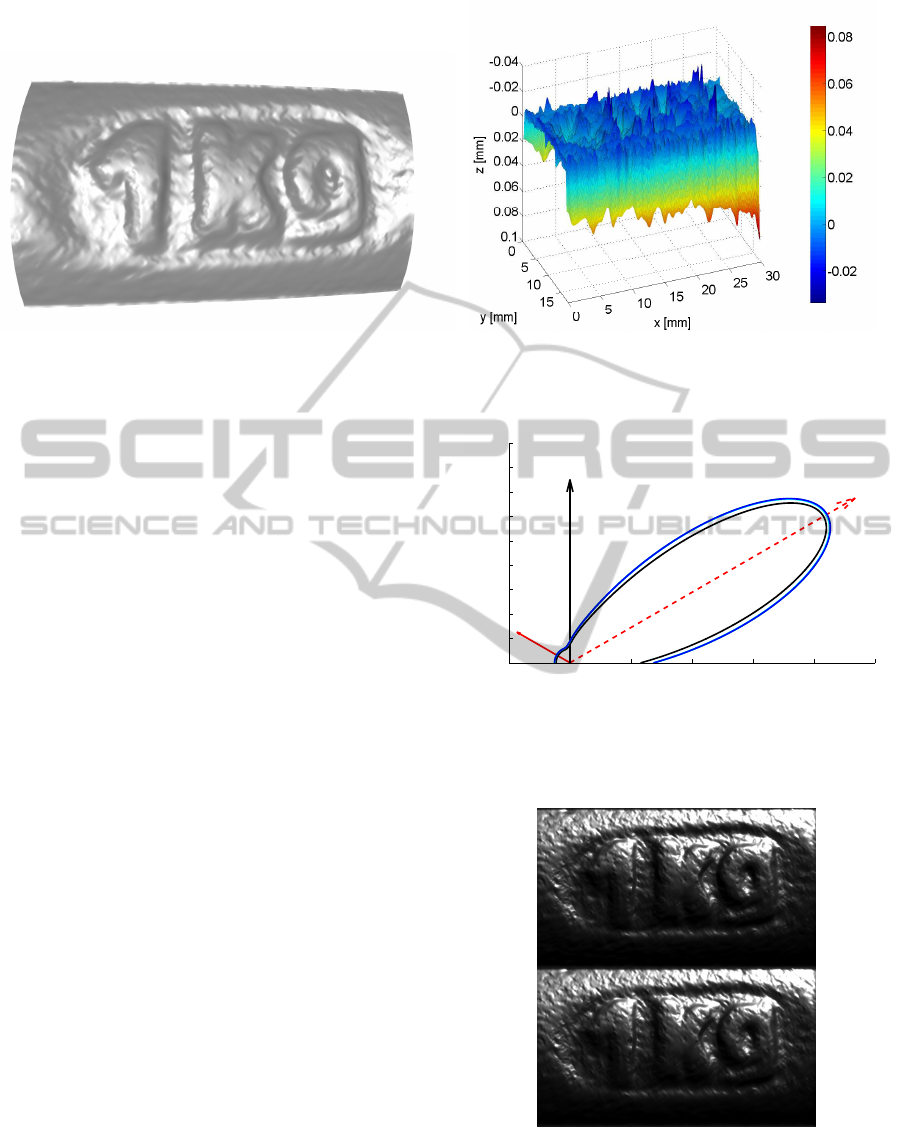
(a) Reconstruction result using synthetic data for validation. (b) Deviations of the reconstructed surface from the synthetic ground truth.
The RMSE amounts to 10.2µm
Figure 5: Validation of the proposed algorithm based on synthetic ground truth data.
used for 3D reconstruction as the SSIM corresponds
to a very high value of 0.985 on the full resolution
scale (cf. Fig. 7).
5 SUMMARY AND
CONCLUSIONS
In this study, we have described an approach that
provides a detailed 3D surface reconstruction along
with simultaneously estimated parameters of the re-
flectance model based on a combination of active
range scanning data for large-scale accuracy with
image-based photometric information for small-scale
accuracy. The simultaneous estimation of the 3D sur-
face profile and the reflectance model is incorporated
into a self-consistent computational scheme that suc-
cessively increases in resolution. We have presented
results for a dark rough metallic surface, which has
been reconstructed based on a single coarse 3D scan
and 12 images acquired under different illumination
conditions. The experimental evaluation has shown
that the obtained surface exhibits a high level of visi-
ble detail. A comparison of a depth difference on the
reconstructed 3D surface profile with a simple tac-
tile measurement has shown deviations of the order
of some 10 µm, while a validation based on synthetic
image data has revealed a RMSE of 10.2 µm or about
1/4 of the lateral extent of a pixel. However, a better
validation of the absolute accuracy is still required,
e.g. using data from a highly precise tactile measure-
ment device.
Additionally, it has been shown that the applica-
tion of a parametric reflectance model allows to de-
termine the reflectance parameters along with the re-
constructed surface. Since the estimated strengths of
−50 0 50 100 150 200 250
0
20
40
60
80
100
120
140
160
180
observed intensity (x component)
observed intensity (y component)
Figure 6: Full reflectance function determined using syn-
thetic data. Black: ground truth; blue: 4 sub-iterations.
There are no differences visible within the thickness of the
blue line for 1 and 2 sub-iterations.
Figure 7: Full-scale synthetic image (top) and correspond-
ing reflectance map (bottom) of the reconstructed surface.
The SSIM amounts to 0.985, thus indicating a very high
similarity.
the specular lobe and the specular spike already in-
crease with increasing resolution level, it might be fa-
VISAPP 2012 - International Conference on Computer Vision Theory and Applications
120

vorable to choose a more suitable reflectance model
or to use a data-driven, non-parametric approach to
model the observed complex behaviors and/or to ac-
quire images from several viewpoints. Nevertheless,
the accurate 3D reconstruction results show that the
applied reflectance function is suitable for integrating
the image-based photometric information with the ab-
solute depth data.
A somewhat critical aspect lies in the generaliza-
tion of the presented approach with regard to inter-
reflections. Currently, the algorithm assumes only
first-order reflections, which induces errors if inter-
reflections occur. Hence, future work will address the
development of a mechanism for the compensation
or the exploitation of the effects of interreflections at
specular surfaces.
REFERENCES
Beckmann, P. and Spizzichino, A. (1987). The Scattering of
Electromagnetic Waves from Rough Surfaces. Num-
ber ISBN-13: 987-0890062382. Artech House Radar
Library.
Cook, R. L. and Torrance, K. E. (1981). A reflectance model
for computer graphics. Proceedings of the 8th an-
nual conference on Computer graphics and interac-
tive techniques, 15(3):307 – 316.
Herbort, S., Grumpe, A., and W
¨
ohler, C. (2011). Re-
construction of non-lambertian surfaces by fusion
of shape from shading and active range scanning.
ICIP’2011, pages 1–4.
Horn, B. K. P. (1970). Shape from shading: A method for
obtaining the shape of a smooth opaque object from
one view. Technical Report 232, Messachusets Insti-
tute of Technology.
Horn, B. K. P. (1989). Height and gradient from shading.
Technical Report 1105A, Massachusetts Institute of
Technology, Artificial Intelligence Laboratory.
Lafortune, E. P. F., Foo, S.-C., Torrance, K. E., and Green-
berg, D. P. (1997). Non-linear approximation of re-
flectance functions. SIGGRAPH’97, pages 117–126.
Lambert, J.-H. (1760). Photometria, sive de mensura et
gradibus luminis, colorum et umbrae. Vidae Eber-
hardi Klett.
Lensch, H. P. A., Kautz, J., Goesele, M., Heidrich, W., and
Seidel, H.-P. (2003). Image-based reconstruction of
spatial appearance and geometric detail. ACM Trans-
actions on Graphics, 22(2):234–257.
Lewis, R. R. (1994). Making shaders more physically plau-
sible. Fourth Eurographics Workshop on Rendering,
pages 47–62.
Matusik, W., Pfister, H., Brand, M., and McMillan, L.
(2003a). A data-driven reflectance model. ACM
Transactions on Graphics, 22(3):759–769.
Matusik, W., Pfister, H., Brand, M., and McMillan, L.
(2003b). Efficient isotropic brdf measurement. ACM
International Conference Proceeding Series (Pro-
ceedings of the 14th Eurographics Workshop on Ren-
dering), 44:241–247.
Mor
´
e, J. J. (1978). Lecture Notes in Mathematics - Nu-
merical Analysis (Proceedings of the Biennial Con-
ference Held at Dundee, volume 630, pages 105–116.
Springer.
Nayar, S. K., Ikeuchi, K., and Kanade, T. (1990). Determin-
ing shape and reflectance of hybrid surfaces by photo-
metric sampling. IEEE Transactions on Robotics and
Automation, 6(1):418–431.
Nehab, D., Rusinkiewicz, S., Davis, J., and Ramamoor-
thi, R. (2005). Efficiently combining positions and
normals for precise 3d geometry. ACM Transactions
on Graphics (Proceedings of ACM SIGGRAPH 2005),
24(3):536–543.
Phong, B. T. (1975). Illumination for computer generated
pictures. Communications of the ACM, 18(6):311 –17.
Wang, Z., Bovik, A. C., Sheikh, H. R., and Simoncelli, E. P.
(2004). Image quality assessment: From error visi-
bility to structural similarity. IEEE Transactions on
Image Processing, 13:600–612.
Ward, G. J. (1992). Measuring and modeling anisotropic
reflection. ACM SIGGRAPH Computer Graphics,
26(2):265–272.
Weyrich, T., Lawrence, J., Lensch, H., Rusinkiewicz, S.,
and Zickler, T. (2008). Principles of appearance ac-
quisition and representation. ACM SIGGRAPH 2008
classes, none:1–70.
W
¨
ohler, C. and d’Angelo, P. (2009). Stereo image analysis
of non-lambertian surfaces. International Jounal of
Computer Vision, 81(2):529–540.
Woodham, R. J. (1980). Photometric method for determin-
ing surface orientation from multiple images. Optical
Engineering, 19(1):139–144.
SELF-CONSISTENT 3D SURFACE RECONSTRUCTION AND REFLECTANCE MODEL ESTIMATION OF
METALLIC SURFACES
121
