
A POLYHEDRAL APPROACH TO COMPUTE
THE GENUS OF A VOLUME DATASET
D. Ayala, E. Verg´es and I. Cruz
Department de Llenguatges i Sistemes Inform`atics, Universitat Polit`ecnica de Catalunya, Barcelona, Spain
Keywords:
Binary Volume Models, Orthogonal Pseudo-polyhedra, Euler Characteristic, Genus.
Abstract:
Topological characteristics are fundamental in many areas. In this paper wepresent a method that computes the
Euler characteristic and the genus of a volume dataset. The followed approach, based on the analogy between
binary volume datasets and orthogonal pseudo-polyhedra (OPP), computes the mentioned values using two
models that are suitable for representing OPP: the Extreme Vertices Model (EVM) and the Ordered Union of
Disjoint Boxes (OUDB). We show the results of these methods for phantom models as well as real datasets,
and compare the efficiency of the presented methods with those based on the classic voxel model.
1 INTRODUCTION
The measurement of the topological characteristics of
an object such as its number of connected components
and cavities or its genus is a useful tool in many ap-
plications as image analysis. These attributes can be
computed as a way to detect the relevant features of a
model. Alternatively, they can be used to prove that
homotopy is preserved in several kinds of processes,
as skeletonization or simplification. In the Bio-CAD
field, the genus is related to the connectivity which is
used to measure the strength of bones (osteoporosis)
or the quality of biomaterials designed to repair them.
In this paper we present a method for computing
the Euler characteristic (EC) and the genus of a bi-
nary volume dataset. The presented approach con-
siders, first, the non-manifold orthogonal polyhedron
(OP) analog to the binary volume model and, then,
a manifold OP homotopic to the non-manifold one.
After that, the classic method that computes the EC
for polyhedra is applied to the special case of OP. Fi-
nally, the genus is obtained from the EC and the shells
of the model obtained with the application of a con-
nected component labeling (CCL) process. OP are
represented with two alternative models, the Extreme
Vertices Model (EVM) and the Ordered Union of Dis-
joint Boxes (OUDB). EVM is a very concise B-Rep
model for OP while OUDB is a decomposition model.
In this paper, we contrast the results and per-
formance of the presented methods with those that
compute the same parameters using the voxel model.
We use several phantom models and real datasets
for these tests. The main contributions are the
following. First, the implementation of a method
that computes the connectivity for binary datasets as
well as for OP (without voxelizing them), which is
faster than using the reference voxel method. Sec-
ond, it also extends the functionality of the EVM and
OUDB models, which are useful for many operations
such as Boolean, morphological, CCL, or visualiza-
tion (Aguilera, 1998; Rodr´ıguez and Ayala, 2003).
The paper is arranged as follows. Next section re-
views related work. Section 3 introduces the EVM
and OUDB models. Section 4 presents the connectiv-
ity computation method and Section 5 discusses the
achieved results. Finally Section 6 concludes this pa-
per and points out future work lines.
2 BACKGROUND AND RELATED
WORK
2.1 Binary Volume Models and
Orthogonal Polyhedra
A binary volume model is a union of voxels with as-
sociated values restricted to 0 for background voxels
and 1 for foreground voxels. In them, three kinds of
adjacency relations are defined between voxels: 6, 18
and 26-adjacency. Two voxels are 6-adjacent if they
share a face, 18-adjacent if they share an edge or a
face, and 26-adjacent if they share at least a vertex.
38
Ayala D., Vergés E. and Cruz I..
A POLYHEDRAL APPROACH TO COMPUTE THE GENUS OF A VOLUME DATASET.
DOI: 10.5220/0003821400380047
In Proceedings of the International Conference on Computer Graphics Theory and Applications (GRAPP-2012), pages 38-47
ISBN: 978-989-8565-02-0
Copyright
c
2012 SCITEPRESS (Science and Technology Publications, Lda.)
An adjacency pair (m, n) defines the adjacency ap-
plied to a binary volume dataset, meaning that fore-
ground voxels are m-adjacent and background vox-
els are n-adjacent (Kong and Rosenfeld, 1989). Us-
ing the same adjacency relations for foreground and
background voxels results in paradoxes that can be
avoided by restricting these pairs to (6, 26) and (26,
6) (Kong and Rosenfeld, 1989; Lachaud and Montan-
vert, 2000).
Latecki (Latecki, 1997) defines the term of well-
composed. A binary volume model is well-composed
if the configurations shown in Figure 1 (left and mid-
dle), modulo reflections and rotations, are avoided.
He also relates the concepts of well-composedness
with manifoldness. Figure 1 (right) shows the non-
manifold configuration for 2D images.
However, (6, 26) and (26, 6) binary volume mod-
els are non-manifold as 26-adjacency causes non-
manifold configurations on its boundary.
Figure 1: Non-manifold 3D (left and middle) and 2D (right)
configurations.
A polyhedron is a subset of R
3
that is bounded,
closed, regular and semianalytic (Requicha, 1980). A
2-manifold polyhedron can be informally described
as a collection of planar faces such that each edge
is shared only by two faces and each vertex is the
apex of only one cone of faces (Rossignac and Re-
quicha, 1991). A pseudo-polyhedron is an extension
of the concept of polyhedron with a non-manifold
boundary (Tang and Woo, 1991; Rossignac and Car-
doze, 1999). Informally, a pseudo-polyhedron can
be defined as a polyhedron with non-manifold edges
and vertices. A non-manifold edge is adjacent to
more than two faces and a non-manifold vertex is
the apex of more than one cone of faces (Rossignac
and Requicha, 1991). Pseudo-manifolds are equal to
the closure of its interior and are homogeneously 3-
dimensional (Rossignac and Requicha, 1991).
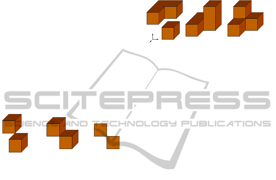
An orthogonal polyhedron (OP) is a polyhedron
with all of its edges and faces oriented in three or-
thogonal directions. The number of faces converg-
ing at OP vertices can be 3, 4 or 6 (Juan-Arinyo,
1995) and we denote by V3, V4 and V6 these kinds
of vertices (see Figure 2). The definition of pseudo-
polyhedra restricted to the orthogonal case results in
that a non-manifold edge is adjacent to 4 faces and a
non-manifold vertex is the apex of two cones of faces.
These two cases are those corresponding to the non-
manifold configurations of Figure 1 (left and middle).
V4
V3
V3
V6
X
Y
Z
Figure 2: Manifold vertices in orthogonal polyhedra: two
configurations for V3 and one for V4 and V6.
The approach followed in this paper uses an or-
thogonal pseudo-polyhedroninstead of a voxel model
to represent a binary volume model as a map be-
tween these two representations can be established
(Khachan et al., 2000). Moreover, as our goal is to
compute the Euler characteristic and the genus us-
ing an expression suitable for manifold polyhedra,
we will convert the orthogonal pseudo-polyhedron
into a manifold one. The basic method to do this
consists in duplicating non-manifold edges and ver-
tices (Floriani et al., 2003). The matchmaker method
(Rossignac and Cardoze, 1999) decomposes a non-
manifold polyhedron into manifold parts by replicat-
ing and bending the non-manifold edges and, then,
replicating and moving slightly apart the remaining
non-manifold vertices. This method minimizes the
number of duplications. Operations of cutting and
stitching (Gu`eziec et al., 2001) are applied to polyg-
onal surfaces to remove non-manifold edges and ver-
tices, for compression purposes. Non-manifold de-
composition has also been extended to general d-
dimensional simplicial complexes (Floriani et al.,
2003). The authors obtain manifold parts for d ≤ 2
and pseudomanifolds parts that require a further de-
composition for d ≥ 3. In (Attene et al., 2009) the
authors justify that tetrahedra models not only have to
be well-shaped but also manifold models in order to
implement efficient methods for Boolean operations
or model simplification. They present an approach for
volume tetrahedral models based on operations that
repair locally first singular edges and then singular
vertices.
2.2 Euler Characteristic and Genus
The Euler characteristic, χ, of a binary volume model
can be expressed in terms of the Betti numbers
(Massey, 1991):
χ = β
0
− β
1
+ β
2
(1)
A POLYHEDRAL APPROACH TO COMPUTE THE GENUS OF A VOLUME DATASET
39

β
i
being the ith Betti number. β
0
and β
2
are asso-
ciated to the number of connected components and
cavities while β
1
is the connectivity which is related
to the genus. χ can be computed from a voxel model
with the following expression (Odgaard and Gunder-
sen, 1993):
χ = n
0
− n
1
+ n
2
− n
3
(2)
n
0
, n
1
, n
2
and n
3
standing respectively for the num-
ber of vertices, edges, faces and voxels. β
0
and β
2
are
usually computed using a CCL algorithm and χ and
the connectivity β
1
with expressions 2 and 1, respec-
tively. Toriwaki et al. present two different strategies
to compute expression 2 and allow several adjacency
pairs (Toriwaki and Yonekura, 2002).
Moreover, in the solid modeling area, χ can be
computed from a polyhedron with the following ex-
pression (Mantyla, 1988):
χ = V − E + F − R = 2(S− g) (3)
V,E, F and R being the number of vertices, edges,
faces and internal rings of faces, respectively, of a
polyhedron. S is the number of shells (number of sets
of connected faces) and g is the genus.
For the special case of triangulated surfaces, χ can
be expressed as:
χ = V − E + T (4)
V, E and T being the number of vertices, edges and
triangles of the mesh.
A triangle mesh can be extracted from a voxel
model to approximate a given isosurface separating
interior and exterior voxels. This mesh can be ob-
tained with the Marching Cubes algorithm (Lorensen
and Cline, 1987) or one of its derived methods that
try to solve the flaws of cracks and ambiguities of the
initial proposal (Bourke, 1994).
Expression 4 is combined with Expression 1 to
compute the connectivity of a triangular isosurface
corresponding to the Laplacian of the electron density
field of adenine (Konkle et al., 2003). In this case, β
0
and β
2
are computed with a CCL method applied to
triangular surfaces. An incremental method is used to
compute the Betti numbers for any dimension as well
as for α-shapes (Delfinado and Edelsbrunner, 1993).
The Euler characteristic and genus are used to de-
termine if two objects have the same topology. In-
formally, two objects are homotopic, i.e., have the
same topology, if they have the same number of con-
nected components, tunnels and cavities (Kong and
Rosenfeld, 1989). Homotopy is a desirable property
in many methods and applications such as thinning.
The concepts of simple voxel and simple deforma-
tions are also used to define topology preservation for
skeletonization and to devise the corresponding thin-
ning methods, based on the deletion of simple vox-
els (Rosenfeld et al., 1998; Bertrand and Malandain,
1994; Borgefors et al., 1999). In isosurface extrac-
tion, topology-preservation is sometimes a desirable
property that can be evaluated by computing the Eu-
ler characteristic (Schaefer et al., 2007). Sarioz
et al. (Sarioz et al., 2004) compute the Betti num-
bers β
0
, β
1
and β
2
with a fast incremental approach.
They use these triples, computed for the binary vol-
umes obtained from every possible threshold value of
a gray-scale 3D image, to classify a large collection
of datasets.
In the Bio-CAD field, the connectivity is related to
biomechanical properties and is used to measure the
strength of bone or other materials. The method based
on expressions 1 and 2 is used to evaluate the osteo-
porosis degree of mice femur (Mart´ın-Badosa et al.,
2003) or human vertebrae (Odgaard and Gundersen,
1993) or to evaluate hydraulic properties of sintered
glass (Vogel et al., 2005).
There are methods that compute the connectivity
from a curve skeleton previouslycomputed. Pothuaud
et al. (Pothuaud et al., 2002; Pothuaud et al., 2004)
apply a 3D-line skeleton graph analysis (3D-LSGA)
to MR images of human vertebrae. The number of
loops of this graph is related to β
1
. Moreover, there
is a relationship between the coordination number of
this graph (average number of edges in a vertex) and
the connectivity (Ioannidis and Chatzis, 2000). Some
other approaches are based on the computation of a
surface skeleton. A plate/rod model is derived, based
on the surface/linear regions of the surface skeleton
(Stauber and M¨uller, 2006; Peyrin et al., 2007) and
the connectivity is measured as the relative amount of
plate and rod elements.
2.3 Alternative Models
Binary volume models are mostly represented with
the classic voxel model. However, in the volume anal-
ysis and visualization field, several alternative models
have been devised for specific purposes.
Hierarchical decomposition models as octrees
and kd-trees have been used for Boolean operations
(Samet, 1990), CCL (Dillencourt et al., 1992), thin-
ning (Quadros et al., 2004) and also to extract and
simplify isosurfaces (And´ujar et al., 2002; Vander-
hyde and Szymczak, 2008; Greβ and Klein, 2004).
Other models aim to store only surface voxels to
gain storage and computational efficiency. The semi-
boundary representation allows direct access to sur-
face voxels and performs fast visualization and ma-
nipulation operations (Grevera et al., 2000). There
GRAPP 2012 - International Conference on Computer Graphics Theory and Applications
40
are methods for morphological operations and CCL
that use this representation (Thurfjell et al., 1995).
The slice-based binary shell representation also stores
only surface voxels and is applied to render binary
volumes (Kim et al., 2001).
3 EVM AND OUDB
REPRESENTATIONS
In this work, the Euler characteristic and the genus are
computed using two alternative representations. This
section introduces the EVM and OUDB models. For
a deeper study of these models and their properties,
see (Aguilera, 1998) and (Rodr´ıguez et al., 2004).
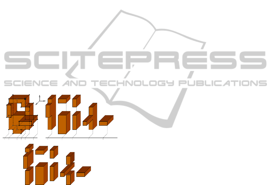
The Extreme Vertices Model (EVM) is an implicit
B-Rep model for orthogonal pseudo-polyhedra that
stores only a subset of its vertices, named extreme
vertices (EV). These vertices are the ending vertices
of maximal uninterrupted segments (see Figure 3)
which are stored lexicographically.
C4C5 S1 S2 S3 S4 S5
X
Z
Y
C1 C6C3C2
A B
Figure 3: Above, left: an orthogonal pseudo-polyhedron
with 38 marked extreme vertices and 6 cuts. Above, right:
its sequence of 5 prisms with the representative section (X
direction). Below: Its XY OUDB representation. Note that
EVM only stores the extreme vertices A and B in the cor-
responding marked line AB, that also crosses three more
internal vertices (two V4 and one V6 that are not stored in
the EVM).
A cut, C
i
, is the set of extreme vertices lying on
the same orthogonal plane (see Figure 3, above, left).
An orthogonal polyhedron can also be seen as a se-
quence of orthogonal prisms represented by its sec-
tion, S
i
(see Figure 3, above, right). Cuts and sections
are orthogonal polygons embedded in 3D space. For
each main direction, sections can be computed from
cuts and cuts from sections with the two following ex-
pressions: S
i
= S
i−1
⊗C
i
, S
0
=
/
0 and C
i
= S
i−1
⊗ S
i
,
i = 1..n. The symbol ⊗ stands for the XOR Boolean
operation.
These operations are actually performed on the
projections of cuts and sections onto the main plane
parallel to them. So, from now on, we denote as C
i
and S
i
the projection of the ith cut and the ith section
respectively onto the main plane parallel to them.
Moreover, there is a property concerning orthog-
onal polygons and polyhedra represented with EVM
that states that the XOR Boolean operation is reduced
to the application of an XOR at the vertices’ level
(0-D XOR). EVM(A ⊗ B) = EVM(A) ⊗ EVM(B).
Therefore the computation of sections from cuts and
cuts from sections is a simple XOR of its vertices.
The Ordered Union of Disjoint Boxes (OUDB) is
a decomposition model that is derived from EVM by
splitting the aforementioned orthogonal prisms into
boxes (see Figure 3, below). OUDB is axis-aligned as
octrees and bintrees but the partition is done along the
object geometry like the BSP model. In the presented
approach, to compute the genus, we will use a CCL
method developed for the OUDB model (Rodr´ıguez
and Ayala, 2003).
The improved performance achieved with these
alternative representations relies on the fact that the
corresponding algorithms are basically traversals of
extreme vertices or boxes instead of traversals of vox-
els and that, in most cases, the number of extreme ver-
tices and boxes is substantially smaller than the num-
ber of foreground voxels.
Many operations have been developed for these
models and some of them are used in the pre-
sented approach as morphological erosion and dila-
tion (Rodr´ıguez and Ayala, 2003). These operations
are recursive in the dimension and are actually per-
formed on the 1D sections of the 2D sections of the
aforementioned prisms.
4 COMPUTATION OF THE
EULER CHARACTERISTIC
AND GENUS
The approach followed in this paper to compute the
Euler characteristic and the genus is based on expres-
sion 3, suitable for manifold polyhedra. As the con-
tinuous analog of a (26, 6) or (6, 26) binary volume
model is an orthogonal pseudo-polyhedron, we will
convert it into a manifold one with an offset opera-
tion.
A positive offset is defined as (Rossignac and Re-
quicha, 1986):
P
′
= P⊕ d = {p | ∃q ∈ P,dist(p,q) ≤ d} (5)
A POLYHEDRAL APPROACH TO COMPUTE THE GENUS OF A VOLUME DATASET
41
dist can be computed in several metrics. In this
paper, we use the chessboard metric, L
∞
, to guaran-
tee the closure of orthogonal polyhedra under offset
operations.
A negative offset is defined as the complement of
the expanded complement. Positive and negative off-
sets are related respectively to dilation and erosion
(Gonzalez and Woods, 1992) and to Minkowski sum
and decomposition (Ghosh and Haralick, 1996).
Then, our method is supported by the following
proposition:
Proposition 1 Let P be an orthogonal pseudo-
polyhedron that is the continuous analog of a (26, 6)
binary volume model and let P
′
be the positive offset
of P with distance d < 0.5s, P
′
= P ⊕ d, and s be-
ing the voxel’s size of the underlying binary volume
model. Then, the two following properties hold:
• P and P
′
are homotopy-equivalent
• P
′
is a 2-manifold
This proposition is now demonstrated informally.
With the positive offset, we duplicate all the non-
manifold edges and vertices topologically as well as
geometrically and this is the basic process to con-
vert a non-manifold to a manifold. However, a non-
restricted positive offset could result in new connec-
tions or disconnections of the boundary of P and,
therefore, the resulting offset would have a differ-
ent number of connected components, cavities or
tunnels than the original object. Even worse, new
non-manifold elements could appear in other regions.
Both problems are avoided if the offset distance is less
than half the size of the voxel of the underlying binary
volume model.
An analogous proposition can be stated for (6, 26)
binary volume models, in which case a negative offset
is applied.
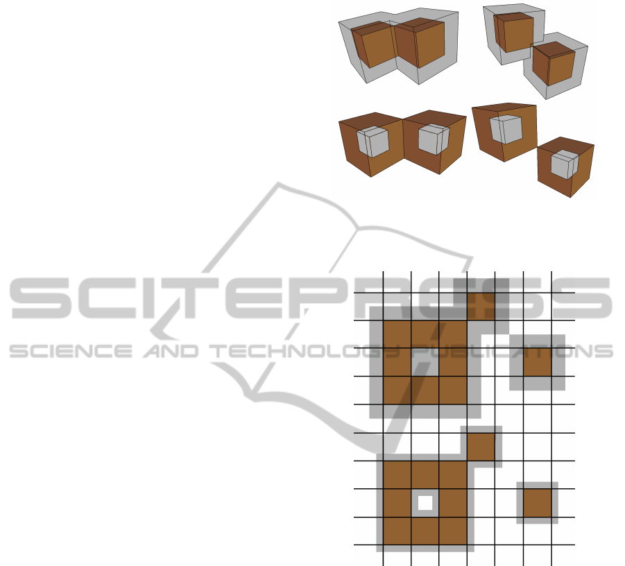
Figure 4 (above) shows the result of applying a
positive offset to two orthogonal pseudo-polyhedra
that include the two possible non-manifold configura-
tions (edge and vertex). Figure 4 (below) is analogous
for a negative offset.
Figure 5 shows a 2D example with an orthogonal
polygon and the underlying binary model. The initial
polygon (in brown) has 2 connected components and
1 hole. Above, we apply a positive offset with d =
0.5s and the resulting polygon has only one connected
component and no holes. Moreover, with this offset
a non-manifold vertex has disappeared but a new one
has been created. With d < 0.5s (below) the resulting
polygon is homotopy-equivalentto the initial one, the
non-manifold vertex has been removed and no new
non-manifold vertices have appeared.
The proposed method uses alternatively the
EVM and OUDB representations of the polyhedron
Figure 4: Positive (above) and negative (below) offsets
applied to the non-manifold configurations of orthogonal
pseudo-polyhedra. In brown, the initial polyhedron.
Figure 5: A 2D example showing the result of applying a
positive offset with d ≥ 0.5s (above) and d < 0.5s (below).
(EVM-Rep and OUDB-Rep) that have already
been computed. The whole process consists of the
following steps, that are explained below:
Input: EVM-Rep and OUDB-Rep of the polyhedron
Output: Euler characteristic (χ) and genus (g)
1. Compute the number of connected components
from OUDB-Rep, n1
2. Compute the complement of OUDB-Rep
3. Compute the number of connected components of
the complement minus one, n2
4. Compute the number of shells, S = n1 + n2
5. Apply a positive offset with d < 0.5s to the EVM-
Rep
GRAPP 2012 - International Conference on Computer Graphics Theory and Applications
42

6. For each cut,C
i
,i = 1..n, of the dilated EVM-Rep
in each direction X, Y, Z do:
(a) Compute the number of faces, F
i
, (number of
connected components) from the OUDB-Rep
of C
i
(b) Compute the number of rings, R
i
, (number of
connected components of the complement of
the OUDB-Rep of C
i
, minus one)
(c) Detect and count V4
i
and V6
i
vertices
7. Compute the total number of faces (F), rings (R)
and vertices V4 and V6: F = Σ
n
i=1
F
i
, R = Σ
n
i=1
R
i
,
V4 = Σ
n
i=1
V4
i
and V6 = Σ
n
i=1
V6
i
8. V = EV +V4+V6
9. E = (3EV + 4V4+ 6V6)/2
10. χ = V − E + F − R
11. g = S − χ/2
Steps 1, 2 and 3, use a CCL algorithm (Rodr´ıguez
et al., 2004) to compute the number of connected
components (step 1) and the number of cavities (steps
2 and 3). This algorithm follows a classic two-pass
strategy like the algorithms based on voxel models
but it traverses a set of boxes instead of voxels. As
this method can deal with pseudo-manifold polyhe-
dra, it can be applied to the initial object as well as to
the dilated object.
Step 5 applies a positive offset to the EVM-Rep
in order to guarantee that the resulting polyhedron
is a two-manifold. The applied method performs 1-
dimensional offsets consecutively in the three main
directions. The details of the algorithm can be found
in (Rodr´ıguez and Ayala, 2003).
The following steps compute the number of the re-
maining elements in expression 3. We denote by F, E
and R, the number of faces, edges, and internal rings
of faces and by V3, V4, V6 the number of vertices
with 3, 4 and 6 faces converging at them, respectively.
EVM-Rep stores only extreme vertices that, in the
case of manifold polyhedra, coincide with vertices
V3. Therefore,V3 is obtained directly from the EVM-
Rep. To compute F, R, V4 and V6, we perform a
traversal of all the cuts of the EVM-Rep. Every cut is
a 2D orthogonal polygon that is also EVM and OUDB
represented. The faces and rings of a cut (in 2D) play
the same role as the number of connected components
and cavities (in 3D) and so they are computed in the
same way, i.e., by applying the same CCL algorithm.
Therefore, step 6 (a) and (b) are 2D versions of steps
1 to 3.
Step 6 (c) is performed taking into account the
following considerations. Although we are working
with a two-manifold 3D polyhedron, its faces may
present the non-manifold 2D pattern shown in Fig-
ure 1 (right): the two coplanar faces incident to a V4
vertex present this pattern as well as the three pairs
of two coplanar faces of a V6 vertex (see Figure 2).
To compute V4 and V6 we rely on these facts. When
processing each cut, 2D non-manifold vertices are de-
tected and stored in a list together with the number of
times that have been found. V4 vertices are those de-
tected once while V6 are those detected three times.
Detection of 2D non-manifold vertices is per-
formed with EVM-Rep, i.e., with cuts and sections in
1D. When a 1D cut of a polygon contains a vertex of
the previous 1D section, this vertex is non-manifold.
This property is actually evaluated for the projections
of cuts and sections onto the main axis parallel to
them. Figure 6 shows an example of a polygon with
8 cuts and 7 sections. Cut C
7
contains a vertex of sec-
tion S
6
(their projection onto theY axis), therefore the
marked vertex is non-manifold.
C2 C3 C4 C5 C6 C7 C8
Y
X
S1 S2 S3
S4
S5 S6
S7
C1
Figure 6: 2D example with a non-manifold vertex.
Step 7 indicates that all these elements computed
for each cut are added in order to compute F, R, V4
andV6 for the whole object. Step 8 computesthe total
number of vertices (V) and step 9 the total number of
edges (E) from the number of edges that each class
of vertices has: E = (3V3+ 4V4+ 6V6)/2. Finally,
steps 10 and 11 compute the Euler characteristic and
the genus, respectively, using expression 3.
5 RESULTS
We have measured the χ and genus of several test
datasets by means of three methods: the methods ap-
plied to voxel models and to triangle meshes (see Sec-
tion 2.2) and the method applied to EVM/OUDB that
is presented in this paper (see Section 4). These three
methods produce the same results, and in this section
we compare their execution times.
A POLYHEDRAL APPROACH TO COMPUTE THE GENUS OF A VOLUME DATASET
43
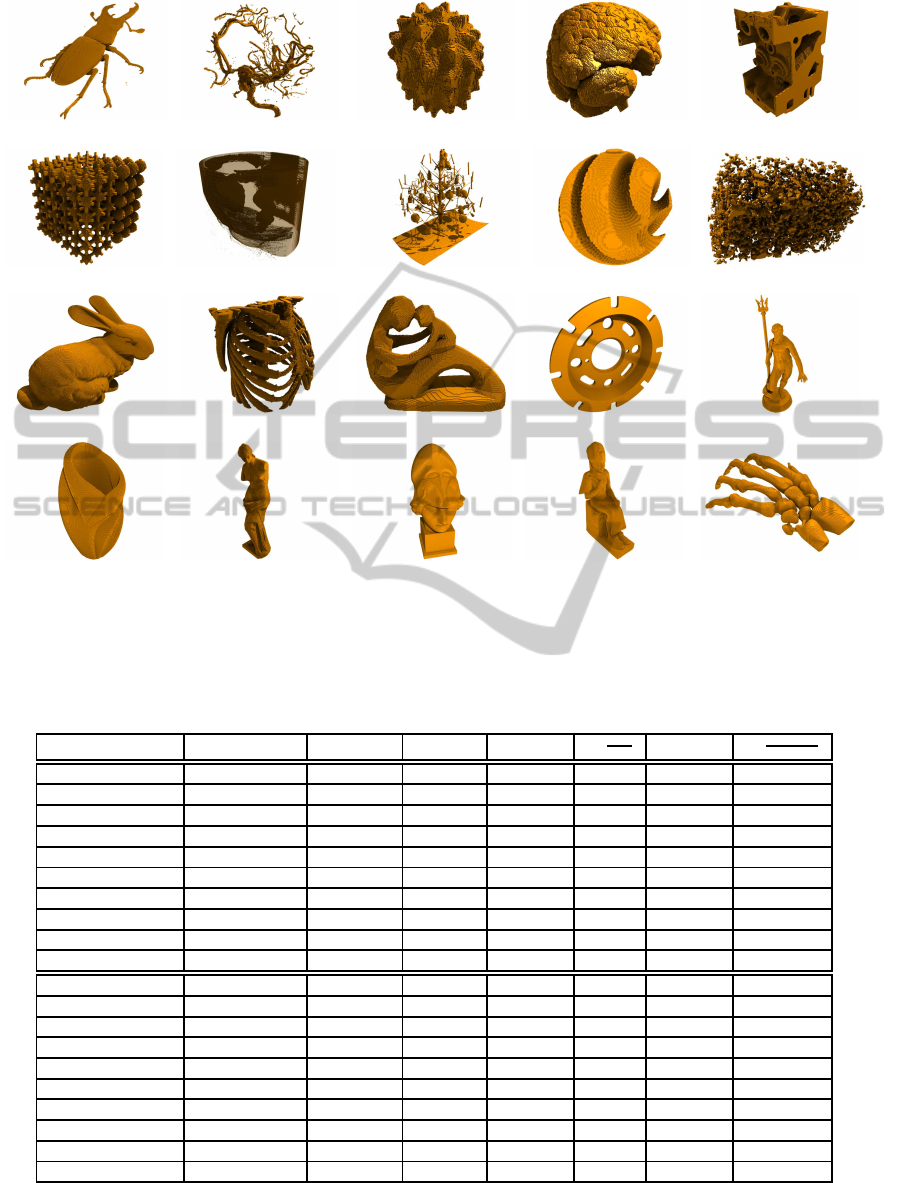
(a) (b) (c) (d) (e)
(f) (g) (h) (i) (j)
(k) (l) (m) (n) (o)
(p) (q) (r) (s) (t)
Figure 7: Rendered images of test datasets.
Table 1: For each tested dataset, the size of the voxel model, number and percentage of internal voxels, number of extreme
vertices in the EVM-Rep, ratio between extreme vertices and internal voxels, and number of triangles of the triangle mesh
isosurface extracted with MC.
Name size int. v. % int. v. EV %
EV
intv.
triangles %
EV
triangles
(a) stagbeetle 411x371x247 1737343 4.6 132184 7.6 567972 23.3
(b) aneurysm 213x215x240 69743 0.6 50318 72.1 175064 28.7
(c) daisy 110x113x121 565825 37.6 27570 4.9 125442 22.0
(d) brain 200x250x214 4345477 40.6 240584 5.5 1000222 24.1
(e) engine 139x197x108 901818 30.5 101114 11.2 663900 15.2
(f) scaffold 132x132x132 367632 16.0 89568 24.4 492480 18.2
(g) colon 512x512x426 72625607 65.0 1653726 2.3 7862654 21.0
(h) xmas 459x499x480 801013 0.7 241476 30.1 1574984 15.3
(i) ball 100x100x100 357869 35.8 32348 9.0 133640 24.2
(j) rock 331x211x501 4575786 13.1 821012 17.9 6077500 13.5
(k) bunny 452x331x334 2885577 5.8 437938 15.2 2053328 21.3
(l) chest 314x231x240 1249644 7.2 259604 20.8 1211252 21.4
(m) fertility 232x91x177 862965 23.1 47118 5.5 263200 17.9
(n) disk brake 511x512x73 2584762 13.5 153498 5.9 1150196 13.3
(o) neptune 308x512x227 1754321 4.9 116680 6.7 570788 20.4
(p) vase 139x255x139 825336 16.8 101552 12.3 474812 21.4
(q) venus 148x148x512 3214277 28.7 109184 3.4 559354 19.5
(r) atenea 350x195x512 11758227 33.6 179400 1.5 989988 18.1
(s) ramses 347x999x523 45089181 24.9 426330 0.9 2954748 14.4
(t) hand 511x358x175 1262770 3.9 142828 11.3 654412 21.8
GRAPP 2012 - International Conference on Computer Graphics Theory and Applications
44

Table 2: For each dataset, its number of positive and negative shells, genus and EC and the computation times in seconds for
the methods using the voxel model, the OUDB/EVM-Reps and the triangle mesh.
Name C
+
C
−
genus χ Time χ (s) Time Total (s)
MVoxels EVM MVoxels EVM Mesh
(a) stagbeetle 17 114 226 -190 9.9 0.8 37.1 1.6 2.7
(b) aneurysm 406 12 146 544 3.5 0.4 14.4 0.7 0.2
(c) daisy 1 0 0 2 0.3 0.2 1.1 0.3 0.3
(d) brain 1 542 516 54 3.5 1.4 13.7 3.2 12.1
(e) engine 9 194 130 146 0.6 0.6 2.6 1.3 8.1
(f) scaffold 4 0 256 -504 0.6 0.6 2.1 0.8 1.4
(g) colon 11820 18118 30387 -898 41.2 13.3 178.5 35.1 158.6
(h) xmas 1324 40 171 2386 39.8 1.4 155.2 3.8 4.0
(i) ball 1 0 0 2 2.0 0.1 5.1 0.1 0.4
(j) rock 2502 26 647 3762 10.5 7.1 50.3 31.5 57.0
(k) bunny 1 155 14 284 17.9 2.5 69.2 7.2 16.8
(l) chest 1 106 246 -278 5.7 1.6 23.4 3.7 11.5
(m) fertility 1 0 4 -6 0.7 0.3 3.0 0.5 0.8
(n) disk brake 1 0 11 -20 4.1 0.8 17.6 1.1 7.5
(o) neptune 1 0 4 -6 12.6 1.0 49.8 2.0 2.9
(p) vase 1 0 0 2 1.4 0.6 6.2 1.3 2.5
(q) venus 1 3 4 0 3.4 0.9 13.3 1.8 2.9
(r) atenea 1 30 31 0 9.4 1.4 33.5 2.6 5.0
(s) ramses 1 0 2 -2 56.5 2.2 216.4 4.7 36.3
(t) hand 1 0 5 -8 8.1 1.3 31.7 2.3 2.7
The presented algorithms have been written in C++
and tested on a PC Intel Core 2 CPU E6600 at 2.4
GHz with 3.2 GB and running Linux. All reported
execution times are in seconds.
We have measured the connectivity in a selection
of datasets that encompass a broad range of shape fea-
tures and occupancy ratios. These datasets where ob-
tained from the following public volume repositories:
Aim@Shape, Stanford, S. Roettger, volvis, TU Wien
or own collection.
The volume models are usually provided as
grayscale voxel models that record the density at ev-
ery sampling point in a 3D image. Then, a threshold is
applied to segment the voxels into two groups: back-
ground and foreground voxels.
To obtain a more fair comparison between the
tried methods, the initial voxel models have been re-
duced to match their corresponding minimum bound-
ing box. These resulting datasets present non-
manifold configurations and still contain many iso-
lated cavities and disconnected components.
Figure 7 shows rendered views of the test datasets.
These datasets present a diverse topology: some have
few components (e.g. fertility (m)) but others have
many parts (e.g. xmas (h) or rock (j)); some have few
tunnels (e.g. bunny(k)) and others many of them (e.g.
scaffold (f)); some contain visible cavities (e.g. colon
(g)) but others do not (e.g. ramses (s)); some present a
simple geometry with few faces (e.g. vase (p)) whilst
others are more intricate (e.g. chest (l)).
We consider that the EVM/OUDB representations
are available and ignore the cost of conversion from
and to a voxel model (which is less than 10 seconds
for most datasets and less than 120 s. for the larger
ones. Similar times appear for the conversion to tri-
angle meshes using Marching Cubes). Nevertheless,
these EVM/OUDB conversion algorithms have also
been published (Aguilera and Ayala, 2001; Rodr´ıguez
et al., 2004).
Table 1 shows the characteristics of the datasets:
the size of the voxel model, the number and percent-
age of internal voxels, the number of extreme ver-
tices of the corresponding EVM-Rep, the ratio be-
tween internal voxels and extreme vertices, the num-
ber of triangles of a triangular surface mesh obtained
via Marching Cubes and the ratio between triangles
and extreme vertices. Note how the equivalent repre-
sentation of a binary model as an EVM usually pro-
vides a large reduction of the number of elements.
Table 2 summarizes the measures of the number of
positive and negativeshells, χ and genus, and the time
needed to compute them using the three referenced
methods, with the best times highlighted.
The time to compute the χ value is negligible
when equation 4 is applied to a triangle mesh, so this
value is not shown in Table 2. Observe that the pro-
posed method is faster than the voxel model reference
method, in some cases up to an order of magnitude.
The difference is smaller if compared with the trian-
gle mesh method: the computation is simpler in that
A POLYHEDRAL APPROACH TO COMPUTE THE GENUS OF A VOLUME DATASET
45

case but it has to process a larger number of elements,
because a triangle mesh extracted with MC generates
a huge number of small triangles.
Also note how the ramses statue, with a boxy
shape, has a very compact encoding as an EVM-
Rep. On the contrary, the aneurysm dataset produces
a quite large EVM, as its internal volume is small and
has many thin features. In this case, the execution
time for the EVM method is worse. The contrary hap-
pens with the xmas tree, which has a very inefficient
voxel model representation as it is almost empty. In
a nutshell, the proposed method behaves better with
very large and compact (not sparse) datasets, such as
the set of scanned statues.
6 CONCLUSIONS AND FUTURE
WORK
In this paper we have presented a method to compute
the Euler characteristic and the genus of a volume
dataset using two alternative models, EVM-Rep and
OUDB-Rep, and we have analyzed their performance
compared to the reference methods applied to voxel
models and triangle meshes.
We have tested several public volume datasets.
We conclude that the connectivity computation in
general is better in the new presented approach with
these test datasets. This improvement is much notice-
able in the complete g computation than in the χ sub-
procedure. The divergence in execution times can be
traced to the size of the datasets but above all to the
intricacy of the represented objects: the method for
voxel models is almost constant time in relation to the
number of voxels, the triangle mesh method mainly
depends on the number of triangles and the proposed
method depends on the number of extreme vertices
of the dataset, with these two latter numbers directly
proportional to the surface tortuosity of the model.
In the biomedical field, there are many other struc-
tural parameters worth to be studied as they describe
the properties of a biomaterial. We have already de-
veloped methods (Verg´es et al., 2008) for obtaining a
pore network. We are now studying other structural
parameters such anisotropy.
We also intend to evaluate temporal sequences
and gray-scale datasets representing real samples with
voxel as well as EVM and OUDB models.
ACKNOWLEDGEMENTS
This work has been partly funded by the CICYT pro-
ject TIN2008-02903 of the Spanish government.
REFERENCES
Aguilera, A. (1998). Orthogonal Polyhedra: Study and Ap-
plication. PhD thesis, LSI-UPC.
Aguilera, A. and Ayala, D. (2001). Geometric Modeling,
volume 14 of Computing Supplement, chapter Con-
verting Orthogonal Polyhedra from Extreme Vertices
Model to B-Rep and to Alternating Sum of Volumes,
pages 1 – 28. Springer.
And´ujar, C., Brunet, P., and Ayala, D. (2002). Topology-
reducing surface simplification using a discrete solid
rep. ACM Trans. on Graphics, 21(2):88 – 105.
Attene, M., Giorgi, D., Ferri, M., and Falcidieno, B. (2009).
On converting sets of tetrahedra to combinatorial and
pl manifolds. Computer Aided Geometric Design,
26:850–864.
Bertrand, G. and Malandain, G. (1994). A new character-
ization of three-dimensional simple points. Pattern
Recog. Lett., 2:169 – 175.
Borgefors, G. B., Nystrom, I., and Baja, G. S. D. (1999).
Computing skeletons in three dimensions. Pattern
Recognition, 32:1225–1236.
Bourke, P. (1994). Polygonising a scalar field.
http://paulbourke.net/geometry/polygonise/.
Delfinado, C. J. A. and Edelsbrunner, H. (1993). An incre-
mental algorithm for betti numbers of simplicial com-
plexes. In SCG’93 Proceedings of the 9th annual sym-
posium on Computational geometry, pages 232–239.
Dillencourt, M. B., Samet, H., and Tamminen, M. (1992).
A general approach to ccl for arbitrary image repre-
sentations. Journal of the ACM, 39(2):253 – 280.
Floriani, L., Mesmoudi, M., Morando, F., and Puppo, E.
(2003). Decomposing non-manifold objects in arbi-
trary dimensions. Graphical Models, 65:2 – 22.
Ghosh, P. K. and Haralick, R. M. (1996). Mathemati-
cal morphological operations of boundary-represented
geometric objects. Journal of Mathematical Imaging
and Vision, 6:199–222. morphological.
Gonzalez, R. C. and Woods, R. E. (1992). Digital Image
Processing. Addison-Wesley.
Greβ, A. and Klein, R. (2004). Efficient representation and
extraction of 2-manifold isosurfaces using kd-trees.
Graphical Models, 66:370 – 397.
Grevera, G. J., Udupa, J. K., and Odhner, D. (2000). An Or-
der of Magnitude Faster Isosurface Rendering in Soft-
ware on a PC than Using Dedicated, General Purpose
Rendering Hardware. IEEE Transactions Visualiza-
tion and Computer Graphics, 6(4):335–345.
Gu`eziec, A., Taubin, G., Lazarus, F., and Horn, B. (2001).
Cutting and stitching: converting sets of polygons to
manifold surfaces. IEEE Transactions on Visualiza-
tion and Computer Graphics, 7(2):136 – 151.
Ioannidis, M. A. and Chatzis, I. (2000). On the Geometry
and Topology of 3D Stochastic Porous Media. Jour-
nal of Colloid and Interface Science, 229:323 – 334.
GRAPP 2012 - International Conference on Computer Graphics Theory and Applications
46

Juan-Arinyo, R. (1995). Domain extension of isothetic
polyhedra with minimal CSG representation. Com-
puter Graphics Forum, 5:281 – 293.
Khachan, M., Chenin, P., and Deddi, H. (2000). Polyhedral
representation and adjacency graph in n-dimensional
digital images. Computer Vision and Image under-
standing, 79:428 – 441.
Kim, B. H., Seo, J., and Shin, Y. G. (2001). Binary volume
rendering using Slice-based Binary Shell. The Visual
Computer, 17:243 – 257.
Kong, T. and Rosenfeld, A. (1989). Digital topology: Intro-
duction and survey. Computer Vision, Graphics and
Image Processing, 48:357–393.
Konkle, S. F., Moran, P. J., Hamann, B., and Joy, K. I.
(2003). Fast methods for computing isosurface topol-
ogy with Betti numbers. In Data Visualization: the
sate of the art proceedings Dagstuhl Seminar on Sci-
entific Visualization, pages 363 – 376.
Lachaud, J. and Montanvert, A. (2000). Continuous analogs
of digital boundaries: A topological approach to iso-
surfaces. Graphical Models, 62:129 – 164.
Latecki, L. (1997). 3D Well-Composed Pictures. Graphical
Models and Image Processing, 59(3):164–172.
Lorensen, W. E. and Cline, H. E. (1987). Marching cubes:
A high resolution 3D surface construction algorithm.
ACM Computer Graphics, 21(4):163–169.
Mantyla, M. (1988). An Introduction to Solid Modeling.
Computer Science Press.
Mart´ın-Badosa, E., Elmoutaouakkil, A., Nuzzo, S., Am-
blard, D., Vico, L., and Peyrin, F. (2003). A method
for the automatic characterization of bone architecture
in 3D mice microtomographic images. Computerized
Medical Imaging and Graphics, 27:447–458.
Massey, W. S. (1991). A Basic Course in Algebraic Topol-
ogy. Springer-Verlag.
Odgaard, A. and Gundersen, H. J. (1993). Quantification of
Connectivity in Cancellous Bone, with Special Em-
phasis on 3-D Reconstructions. Bone, 14:173 – 182.
Peyrin, F., Peter, Z., Larrue, A., Bonnassie, A., and Attali,
D. (2007). Local geometrical analysis of 3D porous
network based on medial axis: Application to bone
micro-architecture microtomography images. Image
Analysis and Stereology, 26(3):179 – 185.
Pothuaud, L., Newitt, D. C., Lu, Y., MacDonald, B., and
Majumdar, S. (2004). In vivo application of 3d-line
skeleton graph analysis (lsga) technique with high-
resolution magnetic resonance imaging of trabecular
bone structure. Osteoporos Int., 15:411 – 419.
Pothuaud, L., Rietbargen, B. V., Mosekilde, L., Beuf, O.,
Levitz, P., Benhamou, C. L., and Majumdar, S. (2002).
Combination of topological param. and bone volume
fraction better predicts the mechanical properties of
trabecular bone. J. of Biomechanics, 35:1091 – 1099.
Quadros, W. R., Shimada, K., and Owen, S. J. (2004). 3d
discrete skeleton generation by wave propagation on
pr-octree for finite element mesh sizing. In Proc.
ACMSymposium on Solid Modeling and Applications,
pages 327 – 332.
Requicha, A. (1980). Representations for rigid solids: The-
ory, methods and systems. ACM Computing Surveys,
12(4):73–82.
Rodr´ıguez, J. and Ayala, D. (2003). Fast neighborhood op-
erations for images and volume data sets. Computers
& Graphics, 27:931–942.
Rodr´ıguez, J., Ayala, D., and Aguilera, A. (2004). Geo-
metric Modeling for Scientific Visualization, chapter
EVM: A Complete Solid Model for Surface Render-
ing, pages 259–274. Springer Verlag.
Rosenfeld, A., Kong, T. Y., and Nakamura, A. (1998).
Topology-preserving deformations of two valued digi-
tal pictures. Graphical Models and Image Processing,
60(1):24 – 34.
Rossignac, J. and Cardoze, D. (1999). Matchmaker: man-
ifold BReps for non-manifold r-sets. In Proc. Fifth
Symposium on Solid Modeling, pages 31 – 40.
Rossignac, J. R. and Requicha, A. A. G. (1991). Contructive
Non-Regularized Geometry. Computer-aided design,
23(1):21 – 32.
Rossignac, J. R. and Requicha, A. G. (1986). Offsetting
operations in solid modeling. Computer Aided Geo-
metric Design, 3:129 – 148.
Samet, H. (1990). Applications of spatial data structures.
Computer Graphics, Image Processing and GIS.
Sarioz, D., Herman, G., and Kong, T. Y. (2004). A technol-
ogy for retrieval of volume images from biomedical
databases*. In Proc. 30th IEEE/EMB Annual North-
east Bioengineering Conference, pages 67–68.
Schaefer, S., Ju, T., and Warren, J. (2007). Manifold dual
contouring. IEEE Transactions on Visualization and
Computer Graphics, 13(3):610 – 619.
Stauber, M. and M¨uller, R. (2006). Volumetric spatial de-
composition of trabecular bone into rods and plates:
A new method for local bone morphometry. Bone,
38(4):475–484.
Tang, K. and Woo, T. (1991). Algorithmic aspects of al-
ternating sum of volumes. Part 1: Data structure and
difference operation. CAD, 23(5):357 – 366.
Thurfjell, L., Bengtsson, E., and Nordin, B. (1995). A
boundary approach to fast neighborhood operations
on three-dimensional binary data. CVGIP: Graphical
Models and Image Processing, 57(1):13 – 19.
Toriwaki, J. and Yonekura, T. (2002). Euler number and
connectivity indexes of a three dimensional digital
picture. Forma, 17:183–209.
Vanderhyde, J. and Szymczak, A. (2008). Topological sim-
plification of isosurfaces in volume data using octrees.
Graphical Models, 70:16 – 31.
Verg´es, E., Ayala, D., Grau, S., and Tost, D. (2008). Vir-
tual porosimeter. Computer-Aided Design and Appli-
cations, 5(1-4):557–564.
Vogel, H. J., T¨olke, J., Schulz, V. P., Krafczyk, M., and
Roth, K. (2005). Comparison of a lattice-boltzmann
model, a full-morphology model, and a pore network
model for determining capillary pressure-saturation
relationships. Vadose Zone Journal, 4:380 –388.
A POLYHEDRAL APPROACH TO COMPUTE THE GENUS OF A VOLUME DATASET
47
