GPU-BASED VISUALIZATION OF HYBRID TERRAIN MODELS

E. G. Paredes

, M. B

, M. Amor

, J. D

ollner

and J. D. Bruguera

Centro de Investigaci

on en Tecnolog

ıas de la Informaci

on (CITIUS), University of Santiago de Compostela,

Santiago de Compostela, Spain

Dept. of Electronics and Systems, Univ. of A Coru

na, A Coru

na, Spain

Hasso-Plattner-Institut, University of Potsdam, Potsdam, Germany

Keywords:

Hybrid Terrain Models, GPU Rendering, Terrain Visualization, Tessellation.

Abstract:

Hybrid terrain models formed by a large regular mesh reﬁned with detailed local TIN meshes represent an

interesting and efﬁcient approach for the representation of complex terrains. However, direct rendering of the

component meshes would lead to overlapping geometries and discontinuities around their boundaries. The

Hybrid Meshing algorithm solves this problem by generating an adaptive tessellation between the boundaries

of the component meshes in real-time. In this paper, we present a highly parallel implementation of this

algorithm using the Geometry Shader on the GPU.

1 INTRODUCTION

Interactive visualization of Digital Terrains Models

(DTM) has been a common subject of research during

the last decade. However, the integration of data from

different sources is still a problematic question, al-

though new data collections are constantly being cre-

ated (Oosterom et al., 2008).

Hybrid terrain models present additional features

for the representation of DTMs, not existing in the

more common regular grid based Digital Elevation

Models (DEM) or Triangulated Irregular Networks

(TIN) models. Using hybrid models, a DTM can be

deﬁned by the combination of regular grid-based ele-

vation data and some locally detailed TIN meshes of

the complete terrain surface representing complex ter-

rain features and artiﬁcial micro-structures like con-

structions or roads. Direct rendering of hybrid terrain

models, however, could generate meshes with holes

and geometric discontinuities between the borders of

the different parts.

The Hybrid Meshing (HM) algorithm (B

oo et al.,

2007) introduces a new method for combining the

TIN and grid meshes in a new coherent crack-free

model, for any LOD in the grid. This approach has re-

cently been extended to support multiresolution ren-

dering of both meshes (Paredes et al., shed).

In this paper, we present the GPU HM method, the

ﬁrst implementation of a hybrid model renderer work-

ing at interactive frame rates into the GPU. Based on

the HM algorithm, our implementation uses Geom-

etry Shader (GS) technology to attain parallelism by

simultaneously running several GS threads perform-

ing the local tessellation of the models boundaries.

2 HM ALGORITHM

The HM algorithm achieves an efﬁcient visualization

of hybrid terrain models formed by a multiresolution

regular grid and local high resolution TINs, as shown

in previous works (Paredes et al., 2009). In Figure

1(c) is depicted an example of the crack-free model

obtained from the union of the view-dependent reﬁne-

ment of a multiresolution grid (see Figure 1(a)) and a

single-resolution TIN (see Figure 1(b)).

The algorithm joins the boundaries of both kind of

meshes following a local tessellation strategy inside

the multiresolution grid cells. The grid cells are clas-

siﬁed as Non Covered (NC), Partially Covered (PC)

or Completely Covered (CC) cells, according to the

overlapping with the TIN mesh. During the visual-

ization, the visible grid cells in the extracted view-

dependent LOD of the grid are processed according

to their classiﬁcation. Thus NC cells are rendered as

usual, CC grid cells are discarded since they will be

replaced by the detailed TIN mesh, and PC cells are

locally tessellated to join both meshes’ boundaries.

To simplify the adaptive tessellation of the cells,

the TIN boundary (TB) is locally convexiﬁed within

254

G. Paredes E., Bóo M., Amor M., Döllner J. and D. Bruguera J..

GPU-BASED VISUALIZATION OF HYBRID TERRAIN MODELS.

DOI: 10.5220/0003823302540259

In Proceedings of the International Conference on Computer Graphics Theory and Applications (GRAPP-2012), pages 254-259

ISBN: 978-989-8565-02-0

 2012 SCITEPRESS (Science and Technology Publications, Lda.)

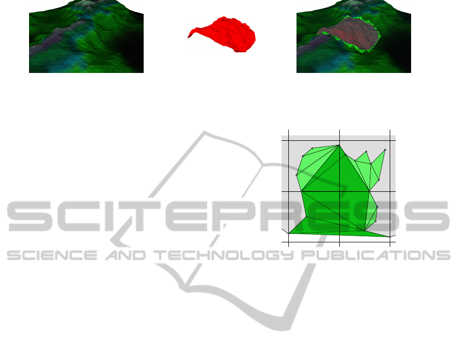
(a) (b) (c)

Figure 1: Hybrid terrain model example. (a) Base regular grid. (b) Detailed TIN component mesh. (c) Resulting hybrid model

with different components highlighted.

each cell in a preprocessing stage, and the result en-

coded in a uniﬁed grid LOD independent representa-

tion. Thus, the convexiﬁcation triangles are decoded

during the visualization, while the remaining PC cells

tessellation triangles are easily generated on-the-ﬂy.

2.1 Local Tessellation Algorithm

Two precomputed data structures are used to connect

the PC cell vertices and the convexiﬁed TIN boundary

inside PC cells: the Grid Classiﬁcation (GC) list and

the list of PC cells (called Vertex Classiﬁcation list in

the original HM article and renamed here for reasons

of clarity). The GC list stores the type (NC, CC, PC)

of each cell in the multiresolution grid mesh. The list

of PC cells contains the information used in the adap-

tive tessellation of each PC cell; i.e., the TB vertices

whose 2D projection falls into the grid cell area, and

the cell corner vertices not covered by the TIN mesh.

Since TB vertices and cell corner vertices are se-

quentially numbered, PC cell related data can be en-

coded as a 4-tuple {A, L, C, I}, where A is the ﬁrst TB

vertex contained in the cell, L is the number of TB

vertices present in the cell, C is the ﬁrst corner vertex

not covered by the TIN mesh, and I is the number of

uncovered corners in the cell. The cell tessellation is

achieved by generating corner triangles joining con-

secutive TB vertices to the uncovered corners of the

cell. Since the TB has been previously convexiﬁed

(see Section 2.2), the cell corner vertices can be safely

joined to consecutive TB vertices, shifting to the next

cell used as link point with the TIN boundary, when

the generated corner triangle overlaps the TIN.

2.2 Incremental Local Convexiﬁcation

of TIN Boundary

To easily regenerate on demand the convexiﬁcation

triangles for a given PC cell of any LOD, the HM al-

gorithm precomputes and encodes these triangles us-

ing a uniﬁed representation valid for every grid LOD.

The process begins by computing the convexiﬁ-

cation of the TIN boundary in the PC cells at the

TIN

Figure 2: Incremental local convexiﬁcation of the TB.

ﬁnest LOD. For each cell, the concave caves on the

TB convex hull are detected and triangulated using

any tessellation algorithm (Shewchuk, 1996). Fig-

ure 2 shows an example (represented in a top view)

where the TB convex hulls of the PC cells are de-

limited by vertices {11, 12, 15} (bottom right cell),

{15, 21, 22} (top right cell), {22, 26} (top left cell)

and {26, 27, 28} (bottom left cell). Once the TIN

boundary convexiﬁcation at this LOD has ﬁnished,

the same process is repeated at the next coarser LOD

until the last one is reached. Since an incremental

convexiﬁcation strategy is used, triangles generated in

this LOD are preserved in the convexiﬁcation of the

next coarser LOD. In the same example of Figure 2,

the convex hull of the coarser level is deﬁned by the

vertices {11, 28}.

The TB list represents the TIN boundary vertices

as a circular list stored in clockwise order. Associ-

ated to each boundary vertex there is an additional

connectivity value indicating the distance, counted in

number of vertices, between that vertex and the most

distant one connected to it in the convexiﬁed TB. If

vertex i has a connectivity value j, the farthest bound-

ary vertex connected to it in the convexiﬁed boundary

is i + j. Also note that the starting vertex of a cave is

connected to all the vertices in that cave, except for

the ones forming part of a nested sub cave. This uni-

ﬁed representation works perfectly well for different

levels of detail, as explained in (B

oo et al., 2007).

GPU-BASED VISUALIZATION OF HYBRID TERRAIN MODELS

255

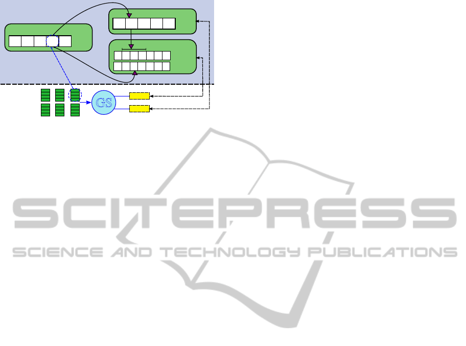
GPU Memory

TB List VBO

tb0

tb1 tb2

tb3

...

TB List

PC Cells VBO

pc0

pc1 pc2

pc3

...

PC List

v1 v2

...

v1 v2

...

TIN

Grid

Geometry VBO

{

Vertex

attributes

TBO

Figure 3: Organization of data structures in memory.

3 GPU HM APPROACH

Our approach attains the parallel tessellation of sev-

eral PC cells by running multiple instances of the HM

algorithm in the GPU cores. Furthermore, an opti-

mized version of the original data structures is used

to improve the memory access.

In our proposal, Geometry Shaders are used to de-

code the precomputed data structures and to generate

the triangles needed for the tessellation of each PC

cell. The GPU parallelism is automatically exploited

as these tasks can be efﬁciently executed simultane-

ously in multicore GPUs.

Next, the optimized data structures and the tessel-

lation and rendering algorithm are presented.

3.1 GPU and CPU Data Structures

The data structures used by the original HM algorithm

were presented in Section 2: the GC list, the list of PC

cells and the TB list. Since in the GPU HM method

the rendering is performed by the Geometry Shader,

every shader thread needs to access some of these

structures and the meshes’ geometric data. The orig-

inal HM data layout, however, can not be efﬁciently

accessed from the GPU. Thus, we have modiﬁed the

data storage and accessing strategies depending upon

their accessing pattern. Figure 3 illustrates the loca-

tion and access methods used for the data structures.

The GC list is only needed to identify the cover-

age pattern of the cell for rendering the grid mesh.

Once the grid cell has been identiﬁed, it is rendered,

discarded or tessellated using the GPU and thus is not

needed by the Geometry Shader.

The GPU HM rendering algorithm uses the geo-

metric data of the TB vertices and the grid cell be-

ing tessellated, together with the TB data and the list

of PC cells. Consequently, these data structures have

to be maintained in GPU memory, stored in Vertex

Buffer Objects (VBO), although they are accessed

in different ways. The geometry data and the TB

list need an array-like access, since the processing

of one PC cell may involve reading non adjacent ele-

ments in random order. Texture Buffer Objects (TBO)

(OpenGL.org, 2009), associated to the correspond-

ing VBOs, are used in our proposal to read this data

within the shader. Using TBOs is an efﬁcient way

to obtain array-like access to large data buffers in the

GPU memory. They provide a convenient interface to

the data, simulating a 1D texture where the tex coordi-

nate corresponds to the offset in the buffer object. Ad-

ditionally, accessing latencies can be effectively hid-

den by overlapping the readings with data processing

operations, since in the HM rendering stage there are

several processing operations.

An additional optimization to improve the data lo-

cality of the TB list has been used. The TIN mesh

vertices are ordered in the vertex buffer containing the

geometry data to guarantee that the TB boundary ver-

tices are stored at the beginning. In this way, the offset

of the vertex data in the buffer object represents its po-

sition in the TB list. Thus, vertex information can be

accessed by using its TB index –reducing one level of

indirection regarding to the original data structures–

and adjacent vertices in the TB are now adjacent in

the buffer object, improving the cache behavior due

to this better data locality.

The PC list, on the other hand, is made avail-

able to the shader through normal input vertex at-

tributes. There is a one-to-one relationship between

PC cells and vertex shader threads; therefore, packing

the items in the PC list as input vertex attributes is the

most effective way to send the right information for

every shader thread. Moreover, data transfer between

CPU and GPU during rendering is reduced, given that

we can use indexed draw calls to select the active PC

cells being tessellated every frame. This list of active

PC cells is easily built on-the-ﬂy by the CPU accord-

ing to the view-dependent grid LOD, and efﬁciently

uploaded to the GPU due to its small size.

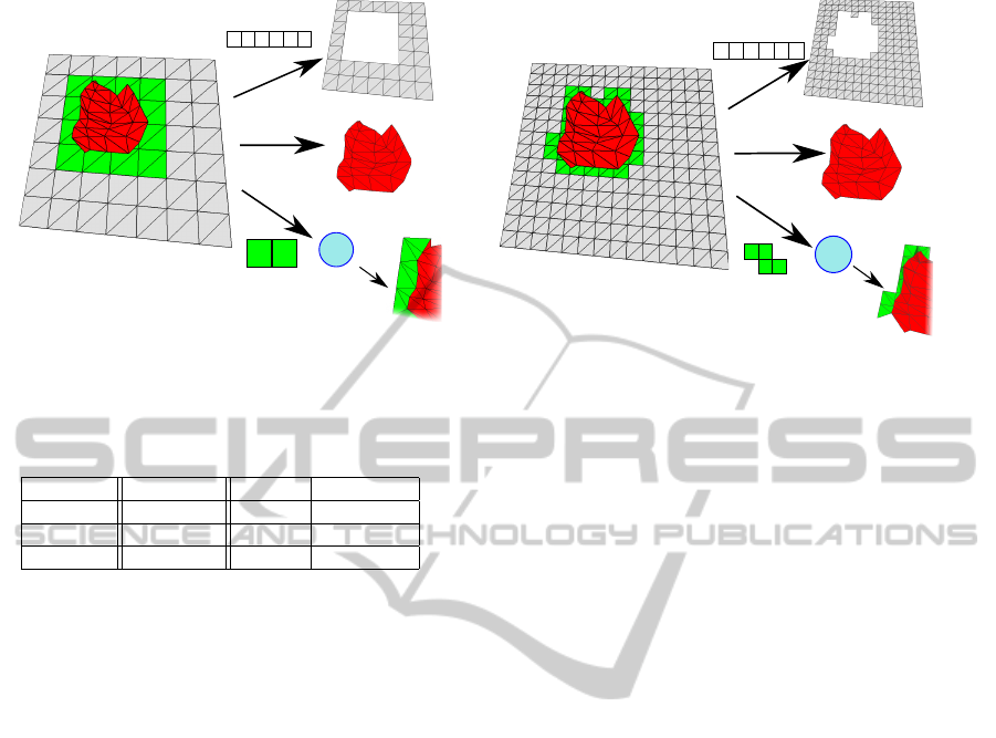
3.2 Rendering Algorithm

The GPU HM rendering steps are similar to the steps

of the original algorithm, but the implementation dif-

fers. An overview of the render ﬂow is presented in

Figure 4 for a coarse (Subﬁgure 4(a)) and a ﬁne (Sub-

ﬁgure 4(b)) grid LOD, following the order of the nu-

merical labels. The TIN mesh is the same in both

cases, but the PC grid cells depend on the grid LOD

and thus different cells are rendered for each case.

The ﬁrst step of the process is to identify the active

NC, CC, and PC cells. Next, the NC cells are ren-

dered using indexed draw calls (step (1) in Figures

GRAPP 2012 - International Conference on Computer Graphics Theory and Applications

256

Vertex Indices

i1 i32

i2 ...

NC cells

TIN

PC cells

PC cells indexes

Step 1

Step 2

Step 3

pc4

pc7

(a)

Vertex Indices

i1 i32

i2 ...

NC cells

TIN

PC cells

Step 1

Step 2

Step 3

PC cells indexes

pc8

pc9

pc2

pc6

(b)

Figure 4: HM rendering algorithm steps. (a) Coarse LOD render. (b) Fine LOD render.

Table 1: Size of the test models.

Model Grid cells TIN ∆ TB elems.

Coru

na 998K 1739K 17K

Sil 998K 657K 14K

Pmouros 998K 656K 16K

4(a) and 4(b)), since geometry data is already stored

in the GPU memory. CC cells are then replaced by

the whole TIN mesh (step (2) in the same ﬁgures).

This operation is lightweight since TIN meshes are

static, usually cover around 20-30% of the grid exten-

sion, and the geometry data are also stored in the GPU

memory, which makes the rendering very efﬁcient.

Finally, the Geometry Shader which performs the

PC cells adaptive tessellation is loaded and the list of

active PC cells are sent to the GPU, where the actual

tessellation is computed (step (3) in the same ﬁgures).

The input of each shader thread is the tessellation data

of the processed PC cell, encoding every data ﬁeld in

a different vertex attribute. By the time the Geometry

Shader ﬁnishes the processing, all the convexiﬁcation

and corner triangles have been generated and the PC

cell is completely tessellated.

During rendering, each one of the running Geom-

etry Shader threads processes the TB vertices in the

cell sequentially. The associated convexiﬁcation tri-

angles are reconstructed and emitted by the Geometry

Shader, according to the algorithm presented in Sub-

section 2.2. Vertices belonging to the local convex

hull of the TIN boundary are connected to the grid cell

vertices, by generating additional corner triangles.

In the GPU HM, the sequential tessellation oper-

ations have been reordered and optimized for GPU

execution. Several techniques have been applied, re-

sulting in an implementation of the algorithm with

fewer conditional branch statements, fewer loops

and a reduced number of memory reading opera-

tions. The implementation strategy presented in (B

et al., 2007) shows that the decoding and generation

of the incremental convexiﬁcation triangles, and the

generation of corner triangles are performed in two

stages. We have succeeded in merging these differ-

ent stages together, reducing the overall complexity of

the source code and the number of conditional evalu-

ations of our implementation.

Additional optimization techniques have been also

used when possible, such as loop unrolling and trans-

formation of complex conditional expressions into

arithmetic expressions or several simpler expressions

for faster evaluation. Another relevant performance

improvement derives from the reordering of the TIN

vertices in the vertex buffer. Due to this optimization,

the data of a TB vertex is accessed with the same in-

dex and in the TB list and in the vertex buffer, elimi-

nating the pointer to the geometry data position used

in the original TB list. With this optimization, not

only are data reading operation reduced to almost one

half of the original number, but also many read op-

erations in the same thread could beneﬁt from data

locality and attain much better cache behavior.

4 EXPERIMENTAL RESULTS

The results of our tests are shown in this section. The

software application used for testing has been coded

in C++. GLSL has been used in the shaders, since

OpenGL is the hardware acceleration API. The per-

formance results were collected in a Ubuntu Linux

system with an Intel Core2 Quad 2.6 GHz proces-

sor. Two different Nvidia GeForce graphic cards, an

GTX480 with 1.5GB of video memory and a GTX280

GPU-BASED VISUALIZATION OF HYBRID TERRAIN MODELS

257

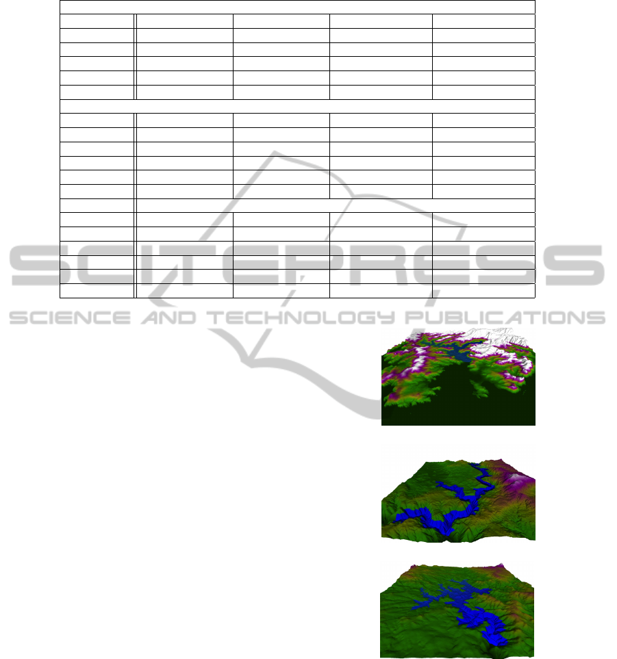
Table 2: Detailed description of the test models composition for each grid LOD.

Coru

L0 L1 L2 L3

PC cells 517 (3.36%) 1058 (1.71%) 2142 (0.86%) 4233 (0.43%)

NC cells 14418 (93.77%) 58606 (94.52%) 236079 (94.81%) 949668 (95.16%)

CC cells 441 (2.87%) 2337 (3.76%) 10780 (4.33%) 44100 (4.42%)

Rendered ∆ 1787K 1876K 2231K 3661K

PC cells ∆ 19K (1,06%) 19K (1,01%) 20K (0,89%) 22K (0,60%)

Sil

L0 L1 L2 L3

PC cells 857 (5.57%) 1775 (2.86%) 3510 (1.41%) 7630 (0.76%)

NC cells 13428 (87.33%) 54666 (88.17%) 217694 (87.43%) 904681 (90.65%)

CC cells 1091 (7.10%) 5560 (8.97%) 27797 (11.16%) 85690 (7.10%)

Rendered ∆ 701K 784K 1111K 2489K

PC cells ∆ 17K (2,38%) 17K (2,17%) 19K (1,66%) 23K (0,90%)

Pmouros

L0 L1 L2 L3

PC 821 (5.34%) 1697 (2.74%) 3329(1.34%) 7912 (0.79%)

NC 13640 (88.71%) 55752 (89.92%) 225396 (90.52%) 906434 (90.83%)

CC 915 (5.95%) 4552 (7.34%) 20276 (8.14%) 83655 (8.38%)

Rendered ∆ 704K 804K 1128K 2497K

PC cells ∆ 20K (2,87%) 36K (4,44%) 20K (1,80%) 27K (1,09%)

with 1GB, were used in the tests.

Three sample models, depicted in Figure 5, were

generated for testing purposes from freely available

data in the Spanish GIS database (IDEE) (Infraestruc-

tura de Datos Espaciales de Espa

na (IDEE), 2002):

Coru

na, Sil and Pmouros. Table 1 contains the size

of the sample models in terms of number of cells in

the ﬁnest LOD of the grids, number of triangles in the

TIN meshes, and number of vertices in the TB.

In Table 2, the number of PC, CC and NC cells are

shown for each grid LOD from L0 − L3 (where L0

represents the coarsest level) as well as its ratio over

the total number of cells. The last two rows show

the total number of triangles used for rendering the

model and the portion of them corresponding to the

adaptive tessellation of the PC cells. Note that the

Coru

na model presents around twice the number of

rendered triangles, as the TIN mesh is much higher

detailed than the others.

The performance results of the GPU HM method

are shown in Table 3. The table shows the averaged

FPS obtained using the HM algorithm are presented

in comparison to the FPS obtained rendering only the

NC grid cells and the TIN mesh, which represents the

maximum theoretical performance of the system. The

relative performance penalty of our implementation is

shown in parentheses. For each sample model, the

tests results are divided according the active LOD in

the grid (L0 − L3).

As can be seen in the results table, the overhead

introduced by the GPU HM implementation does not

prevent the rendering of large terrain models at inter-

(a)

(b)

(c)

Figure 5: Hybrid models used in the tests with the TIN mesh

highlighted in blue. (a) Coru

na model. (b) Sil hybrid model.

active frame rates. The best performance results are

obtained when the coarser LOD (L0) is selected. For

ﬁner LODs, performance tends to decrease, as the to-

tal number of rendered triangles is much higher. The

cost of the HM algorithm implementation, however,

GRAPP 2012 - International Conference on Computer Graphics Theory and Applications

258

Table 3: Performance results obtained with the HM algorithm, measured in FPS, using GTX480 and GTX280 GPUs.

GTX 480

Method L0 L1 L2 L3

Coru

NC + TIN 330.90 319.73 283.64 192.91

HM 232.20 (29.83%) 233.62 (26.93%) 213.31 (24.80%) 155.42 (19.43%)

Sil

NC + TIN 758.97 707.51 561.93 293.89

HM 407.83 (46.27%) 409.74 (42.09%) 353.59 (37.08%) 216.00 (26.50%)

Pmouros

NC + TIN 813.42 754.78 591.35 313.56

HM 276.58 (66.00%) 256.32 (66.04%) 348.41 (41.08%) 210.86 (32.75%)

GTX 280

Method L0 L1 L2 L3

Coru

NC + TIN 90.30 87.99 79.15 62.02

HM 76.06 (15.77%) 87.61 (0.43%) 78.99 (0.20%) 61.82 (0.32%)

Sil

NC + TIN 306.06 283.13 213.35 125.66

HM 196.54 (35.78%) 194.82 (31.19%) 156.93 (26.44%) 101.49 (19.23%)

Pmouros

NC + TIN 354.43 322.90 233.64 134.77

HM 142.74 (59.73%) 148.63 (53.97%) 159.75 (31.63%) 94.43 (29.93%)

is usually higher for coarser grid LODs, which have

a low degree of parallelism. As shown in Table 2,

the number of PC cells nearly doubles for consecu-

tive ﬁner LODs, while the number of PC tessellation

triangles rises only marginally. Since a new parallel

thread is used for the tessellation of a PC cell, this dif-

ference in the number of PC cells directly affects to

the degree of parallelism in the implementation, and

thus the global performance.

This also explains the noticeable larger perfor-

mance penalty when using the more powerful GTX

480 graphic card (480 cores) compared to the GTX

280 (280 cores). Although the absolute performance

is still much better using the GTX 480, the relative

performance of the HM algorithm is worse, since the

GTX 480 has a larger number of cores and thus fewer

threads are being executed by each core. However,

this effect is only important at very high frame rates

and thus it does not limit the validity of our imple-

mentation. For example, our system is able to render

the largest test model, Coru

na bay, at the maximum

available detail (roughly 3.7 millions of triangles) at

155 FPS using the GTX480 card.

5 CONCLUSIONS

The HM algorithm is an efﬁcient solution for render-

ing hybrid terrain models formed by a base multires-

olution grid mesh and high-resolution TINs. In this

paper we have presented a new implementation of

the method based on Geometry Shaders. Due to this

shader based approach, our implementation is easy to

integrate with any modern rendering pipeline.

This GPU implementation of the HM algorithm is

formed by two phases, like the original algorithm.

The harder computations are performed in the pre-

processing phase, and encoded in simple data struc-

tures. During the rendering, the GPU decodes these

structures and generates the adaptive tessellation at

the same time, joining the component meshes.

The performance of the method, as well as the

quality of the rendered hybrid models has been

demonstrated in our experiments. Our implementa-

tion manages to render models of several millions of

triangles, without geometric discontinuities or over-

lapping, at interactive frame rates. To our knowledge,

no other hybrid terrain rendering algorithm has been

implemented using GPUs.

REFERENCES

oo, M., Amor, M., and D

ollner, J. (2007). Uniﬁed hybrid

terrain representation based on local convexiﬁcations.

GeoInformatica, 11(3):331–357.

Infraestructura de Datos Espaciales de Espa

na (IDEE)

(2002). Digital elevation models. http://www.idee.es.

Oosterom, P. v., Zlatanova, S., Penninga, F., and Fendel,

E. (2008). Advances in 3D Geoinformation Systems.

Lecture Notes in Geoinformation and Cartography.

Springer Berlin.

OpenGL.org (2009). OpenGL Texture Buffer Object ext.

Paredes, E. G., B

oo, M., Amor, M., Bruguera, J. D., and

oellner, J. (To be published). Extended hybrid mesh-

ing algorithm for multiresolution terrain models. Int.

Journal of Geographic Information Science.

Paredes, E. G., Lema, C., Amor, M., and B

oo, M. (2009).

Hybrid terrain visualization based on local tessella-

tions. In GRAPP 09: Procs. of the Int. Conf. on Comp.

Graphics Theory and Applications. SciTePress.

Shewchuk, J. (1996). Triangle: Engineering a 2D quality

mesh generator and Delaunay triangulator. Lecture

notes in Computer Science, 1148:203–222.

GPU-BASED VISUALIZATION OF HYBRID TERRAIN MODELS

259