
ON THE REAL-TIME PHYSICS SIMULATION OF A
SPEED-BOAT MOTION
Sergio Casas, Silvia Rueda, José V. Riera and Marcos Fernández
Institute of Robotics, University of Valencia, Valencia, Spain
Keywords: Real-time Simulation, Physics Simulation, Presence, Motion Platform, Virtual Reality, Speed-boat.
Abstract: Training necessities on watercraft have increased during the last few years and real-time simulators offer a
suitable and safe alternative. However, the design of a real-time watercraft simulator implies that, water
simulation and water-vehicle interaction have to be addressed efficiently. This paper presents a simplified
physics model of the water-vehicle interaction for real-time speed-boat simulators that run over 6-DOF
motion platforms. The proposed model is highly parametrizable and can be adapted to any speed-boat by
changing the values of the parameters. We propose the evaluation of the designed model in a quantitative
and a qualitative way. Evaluations results show that the proposed model behaves like a real one in terms of
both objective trajectories and subjective perceived experience.
1 INTRODUCTION
Recent price reduction of simulation hardware and
the irruption of physics-based simulation software,
such as NVidia PhysX (PhysX, 2011), make the
implementation of inexpensive real-time physics-
based realistic vehicle simulators be an increasingly
attainable goal.
Military and civil Virtual Reality (VR) vehicle
simulators have been traditionally linked to training
and pilot instruction. Among the many reasons that
stimulate the research and the use of vehicle training
simulators, the most important ones are the human
and economic costs of the accidents that may occur
if the training process is performed with real
vehicles. Moreover, in watercraft simulation two
reasons are especially relevant: the repeatability and
controllability of the training tests. Wind, swell,
currents, visibility and many other weather-related
variables are almost impossible to predict or enforce,
so the probability of performing a test with the
desired combination of conditions is very limited.
Training necessities on watercraft have increased
during the last few years (mainly because of lower
simulation costs) and some institutions enforce strict
standards for the amount of realism that the
simulators need to provide in order to substitute real
training by simulated sessions (DNV, 2011).
When the problem of simulating watercraft is
studied, the water simulation and the water-vehicle
interaction have to be addressed. Although the two
aspects are intimately related, they are usually
studied separately. Regarding water simulation, the
fluid behavior and its rendering are usually dealt
with separately. With respect to water dynamic
behavior (and fluids in general), we can find a great
deal of studies with many different approaches and
purposes, as the increasing number of conferences
and journals specifically dedicated to this matter
shows. Some works focus on modeling the behavior
of the whole fluid volume with the purpose of
achieving a very realistic model but without interest
in their visual representation. These methods,
usually categorized under the name of
Computational Fluid Dynamics (CFD) (Anderson,
1995), are not usually real-time methods. We can
also distinguish between deep and shallow water
simulation approaches. As shown in (Darles et al.,
2011), the former includes methods that approximate
ocean dynamics with parametric, spectral or hybrid
models and use empirical laws from oceanographic
research. The latter includes physically-based
methods that use Navier–Stokes equations to
represent breaking waves and, more generally, ocean
waves near the shore, using either Eulerian,
Lagrangian or hybrid approaches. Finally, all these
works can be categorized in two distinctive groups,
depending on whether they use superficial or
121
Casas S., Rueda S., Riera J. and Fernández M..
ON THE REAL-TIME PHYSICS SIMULATION OF A SPEED-BOAT MOTION.
DOI: 10.5220/0003823501210128
In Proceedings of the International Conference on Computer Graphics Theory and Applications (GRAPP-2012), pages 121-128
ISBN: 978-989-8565-02-0
Copyright
c
2012 SCITEPRESS (Science and Technology Publications, Lda.)

volumetric representations of the sea (Bulgarelli et
al., 2003). In addition, the selected model will
suggest a corresponding rendering technique.
Since a comprehensive volumetric simulation of
large fluid masses is not, currently, computationally
feasible, surface-based methods are usually selected
for the real-time simulation of oceans. Most of them
discretize analytical equations, defined either in time
or in frequency domains, into meshes. It is advisable
that the implementation uses hierarchical models to
provide more resolution near the floating objects
(Hinsinger et al., 2002).
With respect to watercraft simulation, the
complexity of the water-vehicle interaction has had
an impact on the amount of studies, compared with
other areas, and many of the studies are performed
on large vessels in which the influence of waves is
much lower than in small boats. We could classify
these methods into two categories: classical methods
and system-identification methods. On the one hand,
classical methods use kinematics or dynamics
equations where the velocities or the forces
governing the behavior of the vehicle are described
(Goldstein, 1980). These equations are simplified
and solved, to give the vehicle position and
orientation. On the other hand, system identification
methods try to find a transfer function that could
calculate the vehicle position and orientation from
the inputs of the system (Hann et al., 2010). They
usually work by sampling real inputs from
experiments and measuring the expected outputs.
Then, statistical or heuristic search methods are used
to find a function that suits the sampled data and
could generate suitable outputs when new inputs are
fed.
The purpose of this work is to describe a
physics-based model that could be used to simulate
any kind of speed-boat with a low cost in terms of
CPU usage, while allowing a realistic perception
when used alongside a 6-DoF (Degrees of Freedom)
platform, a visual system and a human interface
system. The CPU usage restriction is achieved by
using a simple but believable approximation and
taking advantage of a state-of-the-art physics SDK
like NVidia PhysX.
The rest of the paper is organized as follows:
Section 2 describes the proposed model for
modeling the physical behavior of speed-boats, the
equations that support it and their rationale. Section
3 describes the tests we performed to achieve an
assessment of our model and the obtained results.
Finally, section 4 shows the conclusions drawn from
our tests, and outlines the future work.
2 PHYSICS MODEL
Before the physics model was designed, different
tests with a real boat were performed in order to set
a qualitative basis for the design of the equations and
to obtain a quantitative description of the required
motion platform design. In these tests, we collected
experimental data of the boat position, speed,
acceleration, tilt, angular speed, angular acceleration
and apparent wind both in time and frequency
domains, by sensorizing a real boat. For the sake of
shortness, the detailed experiments will not be
included here. Although other approaches use this
experimental data in order to find an appropriate
function that suits the data and, therefore, describes
the behavior of the system (Hann et al., 2010), we
consider that an approach based on well-known
rigid-body dynamics and fluid equations could
provide a better approximation. We are not
interested on a particular boat and, even if the tested
vehicle is representative for its kind, it would have
to be proven that a model deduced from one vehicle
is suitable for others. Moreover, the irreproducible
nature of water motion makes impossible to find an
exact comparison between the model and the real
data. Thus, we propose a theoretical approximation
with classical physics equations.
Classical physics tells us that the main forces
describing the behavior of a boat motion are weight,
buoyancy, air friction, water friction and propelling
(either sails or engines) (Palmer, 2005). Some of
these forces, such as air and water drag forces, are
quite complex and an accurate simulation would
require a significant amount of computing time.
However, an excessive simplification would lead to
poor simulation, so a trade-off is necessary.
Therefore, the following assumptions are done:
1- The boat is a rigid body.
2- The ocean surface shape is considered to follow
a known analytic function.
3- The ocean surface shape is not part of the speed-
boat model, it is one of its inputs.
4- The ocean motion influences the boat motion,
and the boat influences the sea surface shape.
5- Wind and swell are considered as a vector.
6- Drag force is calculated as a form drag.
7- Fluid turbulences are ignored.
8- Only helix-based propellers are considered.
Then, the boat is represented by one rigid body,
under the influences of many forces. The shape of
the boat will be described by an adjustable finite
number of small cubes of equal size but different
mass. The exact implementation of each of the
GRAPP 2012 - International Conference on Computer Graphics Theory and Applications
122

aforementioned forces is explained later in this
section.
Although sea-boat interaction is a main key of
the boat motion, our interest is mainly focused on
the boat equations, and not on the sea waves shape.
Indeed, our physics model only needs to know the
sea surface height at any point (to calculate drag
forces and buoyancy). For this reason, we consider
the sea as an input and the influence of the boat on
the sea is left for the sea model. This feature
suggests the use of a surface-based sea model, so
that, we used a superficial sea model to test our
physics model, specifically the one proposed in
(Finch, 2004). In any case, the use of the proposed
physics model is independent from the sea model,
provided that it is possible to calculate the sea height
at any point.
2.1 Vehicle Model
This section describes the forces considered in the
proposed model.
Weight is a downward force that can be
calculated as one resultant force at the center of
mass. However, in order to account for different
material densities and be able to simulate pressure
losses (on inflatable boats), we calculate the weight
of each cube separately as:
= ·
(1)
⋅ : gravity acceleration vector (m/s
2
).
⋅ : cube mass (Kg).
⋅
: weight force (N).
The only adjustable parameter here is m, which
depends on the boat design.
One vertical buoyancy force is calculated for
every cube (Equation 2). As the buoyancy center
changes as the boat displaces water, a distributed
calculation allows us to get a better approximation
of the water volume displaced by the boat and its
resultant buoyancy center.
= · ·
(2)
⋅ : gravity acceleration vector (m/s
2
).
⋅ : submerged volume of the cube (l), calculated
numerically by the intersection of the water line
through the cube.
⋅ : water density (Kg/m
3
), approximated as a
known constant.
⋅
: resultant buoyancy force (N), exerted
upwards at the centroid of the submerged part of
the cube, which is the buoyancy center.
No parameters are found here, as V is variable
and ρ is a constant that does not depend on the boat.
Wind and air drag force are an important part of
the boat behavior. The cube subdivision allows us to
perform a more precise simulation of these effects.
A cube has six faces, and any of the six faces can
resist motion by air drag. Thus, six air drag forces
are calculated at each cube. Air drag accounts for
occlusion with other cubes: if a cube face is
occluded behind another one, air drag is completely
eliminated at that face. This is done in loading time
and it does not need to be calculated every frame.
Wind is not calculated separately, and it is
incorporated into the air drag equation, because in
fact wind and air drag are two parts of the same
effect. The relative speed between the cube face and
the wind vector gives the apparent wind vector
which defines the speed of the air particles at that
particular cube face. Our model also accounts for
other ships wind shadowing by casting rays in
search for occlusions. When an occlusion is detected
at any of the six cube directions, the wind speed is
set to zero (at the corresponding cube face) before
the apparent wind is calculated. Air drag is thus not
eliminated at that face, just the wind effect.
Equations 3 and 4 describe air and wind drag force:
=
(3)
=
1
2
· ·
· ·
·
|
|
(4)
⋅
: fluid (wind) speed vector (m/s).
⋅
: cube speed vector (m/s).
⋅
: apparent wind speed vector (m/s).
⋅ : air density (Kg/m
3
).
⋅
: air drag coefficient.
⋅ : exposed area (m
2
) of the cube face, calculated
numerically by the intersection of the water line
through the cube.
⋅
: resultant air drag force (N).
The only adjustable parameter here is
, that
depends on the fluid, the cube shape and its material;
and it is usually empirically obtained.
Swell and water drag forces are other important
factors when sailing a speed-boat. This calculation is
performed much in the same way as in air. Wind is
substituted by swell, and air by water. Everything
else is analogue, with the difference of density,
because water density is roughly a thousand times
air density. Occlusions also exist. Equations 5 and 6
describe swell and water drag force:
=
(5)
=
1
2
· ·
· ·
·
|
|
(6)
ON THE REAL-TIME PHYSICS SIMULATION OF A SPEED-BOAT MOTION
123

⋅
: fluid (swell) speed vector (m/s).
⋅
: cube speed vector (m/s).
⋅
: apparent swell speed vector (m/s).
⋅ : water density (Kg/m
3
).
⋅
: water drag coefficient.
⋅ : exposed area (m
2
) of the cube.
⋅
: resultant water drag force (N).
Similarly, the only adjustable parameter here is
, which is not necessarily equal to the air drag
constant.
While the engine-helix interaction can be
simulated with a Newtonian approach, the helix-
water interaction and the engine internal functioning
are complex matters that we propose to solve
heuristically. We model the engine as an agent that
generates torque upon the helix. The amount of
torque depends on the input throttle and on the
engine angular speed (Equation 7). This is a
characteristic of combustion engines (Palmer, 2005),
and the exact function is different on each particular
engine. Thus, we consider it as a configurable
parameter. This torque tries to move the engine, but
as it moves, it encounters resistance (Equation 8)
that we model as three terms: a constant friction, a
term that depends on the engine angular speed, and a
term that depends on the engine angular
acceleration. Each term has a corresponding
parameter that controls the amount of each type of
resistance that it is applied to the engine rotor:
,
,
. The result is the net torque.
Engine angular speed is calculated from its
angular acceleration (Equation 9), and angular
acceleration comes from Equation 10. Both
equations come from classical mechanics. The only
parameter in Equations 9 and 10 is , the inertia
matrix, which can be approximated as a constant.
The helix orientation is controlled by the rudder
angle. Although it can be approximated as a linear
function, we implement it as a general function
(Equation 11) that is left as a parameter.
The engine transforms its motion into helix
motion, the helix moves water, and by Newton’s
laws, the water moves the boat (Equations 12 and
13). One revolution of the engine should produce
one revolution on the helix, but as the engine could
be geared, we add a proportionality parameter,
called the differential ratio (
). The helix motion
generates an amount of water displacement that
results in a propelling force. Ideally, one helix turn
produces always the same force and this force is
proportional to the helix shape, dimensions and
angle of attack (Blanke et al., 2000) (Carlton, 2007).
We call this proportionality constant the helix
advance ratio (
). However, turbulences and fluid
slip modify the efficiency of this operation, and not
all the displaced water makes the boat move. In
order to account for that effect we introduce another
parameter that we call helix efficiency, which we
model as a function of the angular speed, because
turbulences and other hydrodynamics effects depend
on the helix speed. This is sometimes referred to as
the slip ratio (Carlton, 2007). The resulting force
calculated at Equation 14 is the propelling force. The
sign is negative because its direction is opposite to
the helix direction. This force is calculated only at
one cube marked as the helix cube.
= (
, )
(7)
=
·
·
(8)
=
·
(9)
=
·
(10)
= ()
(11)
=
·
(12)
= (
|
|
)
(13)
= ·
|
|
·
·
(14)
⋅
: engine angular acceleration (rd/s
2
).
⋅
: engine angular speed (rd/s).
⋅ : engine throttle (range [0..1]).
⋅
: engine torque (N·m).
⋅
: engine constant friction term (N·m).
⋅
: engine speed friction term (Kg·m
2
/s).
⋅
: engine acceleration friction term (Kg·m
2
).
⋅
: engine net torque (N·m).
⋅ : inertia tensor matrix (kg·m
2
).
⋅
: helix angular speed (rd/s).
⋅ : helix efficiency.
⋅ : helix steering angle (rd).
⋅
: helix direction vector (m).
⋅
: engine-helix differential ratio coefficient.
⋅
: helix advance ratio coefficient (Kg/s).
⋅
: resultant engine propelling force (N).
The resultant force at each cube is the sum of all
the former forces (see Equation 15). The application
of all the forces from all the cubes gives a resultant
boat force and a resultant boat torque that can be
transformed successively into acceleration and
angular acceleration, then into speed and angular
speed, and finally into position and orientation. In
our implementation, this calculation is performed by
the NVidia PhysX library. Acceleration and angular
speed are fed into the motion platform, software in
order to create the inertial cues for the simulator.
GRAPP 2012 - International Conference on Computer Graphics Theory and Applications
124
=
+
+
+
+
(15)
3 SIMULATION SETUP
In order to evaluate the proposed physics model, it
was implemented and tested using a complete
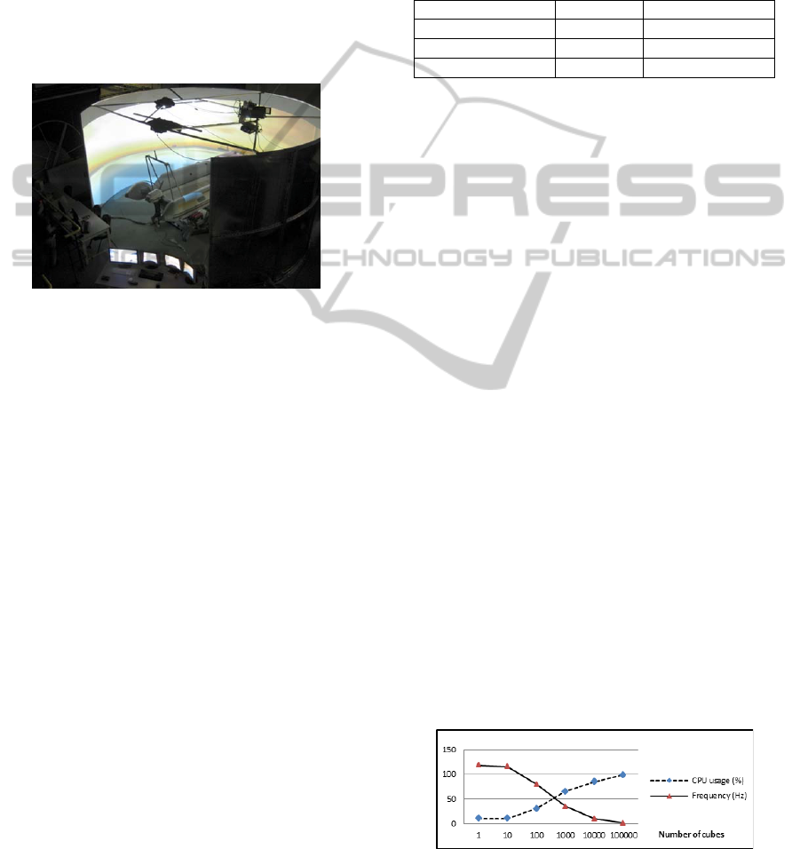
simulator. Figure 1 shows a panoramic of the
hardware layout. Three main elements can be
observed: a cylindrical screen with a projection
system, a 6-DoF motion platform with a sensorized
real speed-boat on it, and an operator console.
Figure 1: Simulator hardware layout.
The projection system consists of a 3m high
cylindrical screen with a diameter of 6 meters
resulting in a 53º vertical and a 270º horizontal field
of view with a total resolution of 3840x1024 pixels.
Sound is also integrated into the simulator in the
form of a 5.1 surround sound system.
The motion platform is a 6-DoF Stewart
(Stewart, 1965) electrical motion platform. It can
handle up to 500 Kg and the excursion limits and
accelerations are shown in Table 1. A motion
platform software module solves the inverse
kinematics of the 6-DoF Stewart motion platform
(Cleary & Brooks, 1993) using a classical washout
algorithm (Reid & Nahon, 1985), (Nahon & Reid,
1990) in order to generate the inertial cues. The
inputs to the washout algorithm (boat linear
acceleration and angular speed) come from the
physics model. In order to create a more immersive
simulation, a real speed-boat was sensorized and
placed on the motion platform.
The visual system, the motion platform, the
operator console, and the sensorized interface are
controlled by a single PC, an Intel Core i7-920
QuadCore, 2700MHz processor with an Asus P6T
Deluxe V2 motherboard, 8Gb of DDR3 memory and
2 NVIDIA GeForce GTX 480 graphic cards with
PhysX support. The OS is a Windows 7 Enterprise.
The proposed physics model has several
parameters that need to be set-up before a valid
assessment can be performed. We can group them in
three groups, the number of cubes for the boat
representation, the physics equations parameters and
those of the washout algorithm. Next sections show
how we have experimentally tuned these parameters.
Table 1: Motion platform excursion limits.
DoF
Excursion
Max. acceleration
Pitch, Roll
25º
±500 º/s
2
Yaw
30º
±500 º/s
2
Heave, Surge, Sway
±0.085 m
±0.5 Gs
3.1 Number of Cubes Set-up
The main purpose of the physics model is to
reproduce the physics behavior of the real boat as
accurately as possible. As the physics model relies
on cube subdivision, the number of cubes is the first
parameter that needs to be addressed.
As the cube subdivision is designed to best suit
the boat shape, the greater the number of cubes, the
more accurate the simulation should be, unless the
CPU usage gets too close to 100%. At that point, the
calculation takes more time than the time-step that is
being simulated, the real-time constraints are broken
and the simulation experience is degraded. However,
if the number of cubes is too small, the simulation
accuracy should also decrease. Therefore, we
intended to find the maximum number of cubes that
the CPU could withstand without losing the real-
time constraints, and that number should maximize
the model accuracy. Given that the physics model is
not the only part of the simulator, a global CPU
usage motorization should be done (and not just a
measure of the physics model performance). The
standard update frequency established as immersion
threshold is 60 Hz (DNV, 2011). So that, we
estimated that the maximum number of cubes that
we could use while maintaining at least a 60 Hz
update frequency over the whole system (both
visual, physics and motion platform) was 549 cubes,
as shown in Figure 2.
Figure 2: Number of cubes vs. CPU update frequency.
ON THE REAL-TIME PHYSICS SIMULATION OF A SPEED-BOAT MOTION
125
3.2 Experts Set-up
Next, we used the previously calculated number of
cubes to set-up the boat model and find appropriate
values for both the physics model and the washout
algorithms parameters. These values were
configured by the consensus of 3 experts on this
kind of vehicles. The configured vehicle tried to
reproduce the behavior of the vehicle on which we
performed the real tests (a Duarry Brio 620
propelled by a Suzuki DF 140 Four Stroke 140 hp
engine). The initial values for the parameters were
set to the theoretical values and then successively
modified in a round-robin-like sequence (one expert,
one modification at a time), until the experts
estimated, by consensus, that the behavior was
plausible. The physics model parameters and their
resulting values are shown in Table 2.
Table 2: Physics model set-up parameters.
Cube densities (inflatable, rigid) [Kg/m
3
]
(150, 500)
Air drag coefficients (x,y,z)
(8,1,6)
Water drag coefficients (x,y,z)
(0.5,7,1)
Engine torque curve function at full
throttle [N·m]
500 rpm: 50,
2000 rpm: 300,
5000 rpm: 500,
7000 rpm: 200
Engine constant friction [N·m]
20
Engine speed friction [Kg·m
2
/s]
2
Engine acceleration friction [Kg·m
2
]
0.1
Engine inertia [Kg·m
2
]
18.5
Steering function (x,y) vector
-60°: (-1,-1),
-30°: (-0.5,-1),
0°: (0,-1),
30°: (0.5,-1),
60°: (1,-1)
Helix efficiency function
500 rpm: 0.8,
2000 rpm: 0.9,
5000 rpm: 0.5,
7000 rpm: 0.2
Engine-helix differential ratio coefficient
1
Helix advance ratio coefficient [Kg·m/s]
1.9
The washout algorithms parameters were set-up
following the guidelines of (Reid & Nahon, 1986)
and are not displayed here for the sake of brevity.
Density was set-up instead of mass, because it
makes easier to change the cubes dimensions. For
simplicity, only two different types of cubes were
considered: those that belong to the rigid part of the
boat, and those that correspond with the inflatable
part. Drag parameters are differentiated in three (one
for each cube face direction). Finally, the functions
were parameterized as piecewise linear functions of
which only a few values are shown.
4 EVALUATION RESULTS
We propose the evaluation of the implemented
model in a quantitative and a qualitative way, so
that, two different set of tests are presented. First, a
quantitative comparison with real data is done to
show whether or not the behavior of the boat
resembles a real one. Then, we need to measure how
immersed users can be in the system. This concept,
known as presence, cannot be analytically measured
and a questionnaire-based expert assessment is
commonly applied (Witmer & Singer, 1998).
4.1 Quantitative Assessment
A quantitative comparison with the real data
(obtained during our experimental tests) was
performed. The tested maneuvers were: 0-25 knots
straight line acceleration, 25-0 knots braking,
sustained 20 knots cruise and 360º turning with
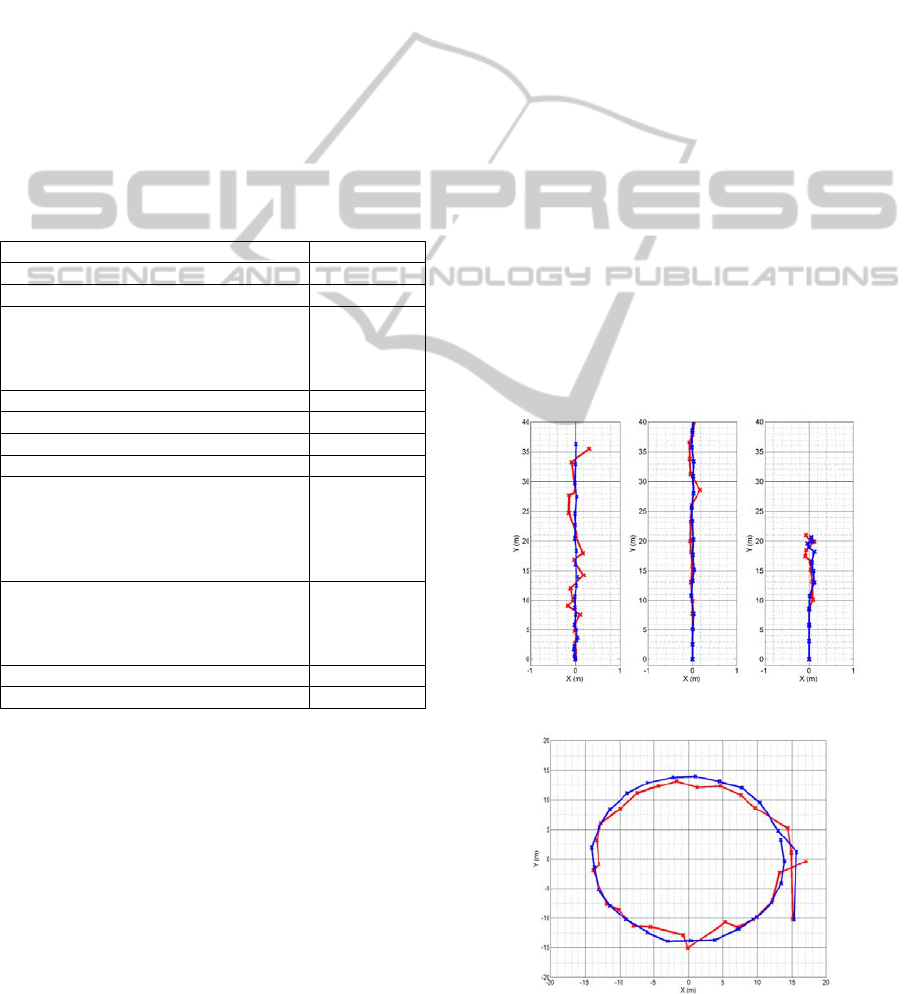
maximum rudder angle. In Figure 3 we can see the
acceleration (left), the constant speed cruise (center)
and the braking (right). Real trajectories are shown
in red and simulated trajectories in blue. Each
marker represents the (x,y) position of the boat ¼
seconds after the previous marker. Similarly, Figure
4 shows a 15 knots full turn.
Figure 3: Full acceleration, cruise, and deceleration.
Figure 4: Full rudder turn.
GRAPP 2012 - International Conference on Computer Graphics Theory and Applications
126
Although the comparison is quantitative, it has to
be carefully interpreted because real environmental
conditions are impossible to reproduce. We can
appreciate that simulated trajectories seem to match
the real ones although real trajectories are a little
noisier. This is probably caused by two reasons: real
sensors are always noisy and real world interactions
are always more complex than the simulated ones,
since the model is a simplification of the real
behavior.
4.2 Experts Assessment
Finally, in order to evaluate the quality of our
solution in terms of presence, 45 experts tested the
simulator (previously configured by a group of three
different experts) in 15 minutes runs. All of them
were asked to perform the same maneuvers on the
same test circuit. The virtual test circuit consisted on
a corridor delimited by two parallel sets of 20
aligned buoys. Each line of buoys was separated by
a distance of 20 meters, and each buoy in the buoy
line was 30 meters away from the next one. The
tested maneuvers were free navigation, 180º turning
at the ends of the buoy corridor, zig-zag sailing
across the two buoy-lines, straight line acceleration,
and constant speed cruise and braking inside the two
buoy-lines.
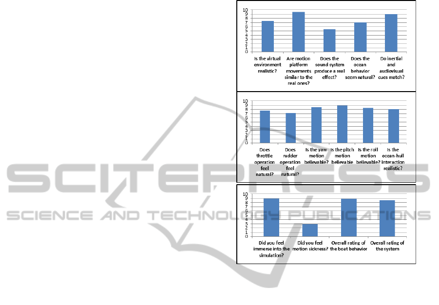
Once they finished the test, they were asked to
fill a questionnaire about their impression. It was
designed following the guidelines explained by
(Jennett et al., 2008). The questions were to be rated
from 0 to 10, with 10 meaning “I totally agree” and
0 meaning “I totally disagree”. We considered that
values greater than 7 meant “it is sufficiently good to
be accepted”, while values lower than 7 meant “it
needs to be improved” (except from motion sickness
that works the other way around). The questions
were grouped in 3 separated blocks. The first block
deals with general questions about the ability of each
module to provide presence and immersion. The
second block of questions is specifically related to
the developed physics model. The third block deals
with the overall impression of the simulator. The
average answers from the 45 questionnaires are
shown in Figure 5.
This results show that, despite some of the
modules certainly need to be improved (such as the
sound system), the overall perception is satisfactory
because the average results are over 8. On the other
side, the specific results of the physics model seem
to be also satisfactory, although some elements like
the rudder operation are felt to be improvable, in the
experts’ opinion. This is probably a consequence of
the absence of actual water resistance while turning
the rudder.
Figure 5: Questions average results.
5 CONCLUSIONS
A simplified real-time model of the dynamics of an
engine-based speed-boat is presented. In order to
obtain an assessment of our model, an evaluation
was performed by introducing our equations into a
complete simulator system. The simulator includes
visual and sound generation, human interface and
real motion generation. The visual system is
rendered on a 270º screen. The inertial cues are
generated by a Stewart 6-DoF motion platform with
a classical washout algorithm.
Since our physics model relies on cube division,
we first calculated the maximum number of cubes
that we could use while maintaining a minimum of
60 Hz. Then, we used this number to find
appropriate values for both the physics model and
the washout algorithms parameters. These values
were configured by the consensus of 3 experts on
this kind of vehicles. At this point, a quantitative
comparison (with real data obtained with our
experimental tests) was performed. We tested a
small number of maneuvers and the virtual
trajectories were similar to the real ones.
ON THE REAL-TIME PHYSICS SIMULATION OF A SPEED-BOAT MOTION
127

Finally, 45 different experts tested the simulator
configured with the previously calculated number of
cubes and the parameters selected by the experts.
Then, they filled a questionnaire about their
impression and their answers showed that the
perceptual error induced by the simplification of the
physics equations and the washout algorithm is low
enough for us to be able to use the simulator for
training purposes.
Future work includes an analytical assessment of
the physics equations by means of an analytical
comparison with real data. A study to find the
optimal number of cubes (the one that maximizes
the ratio presence/CPU usage) could also be
performed. Alternatives to our model, such as
empirical models, can also be studied, designed and
compared. The contribution and correlation of each
of the simulator subsystems (visual system, physics
model, inertial generator, etc) to the overall presence
can also be studied separately. Finally, as our model
is not empirically based, future research could test
the application of the developed equations to
simulate different kinds of vessels.
REFERENCES
Anderson, J.D., 1995. Computational Fluid Dynamics:
The Basics With Applications.
Science/Engineering/Math. McGraw-Hill Science.
Blanke, M., Lindegaard, K.P. & Fossen, T.I., 2000.
Dynamic Model For Thrust Generation Of Marine
Propellers. In 5th IFAC Conference of Manoeuvring
and Control of Marine craft, MCMC'2000., 2000.
Bulgarelli, U.P., Lugni, C. & Landrini, M., 2003.
Numerical modelling of free-surface flows in ship
hydrodynamics. International Journal for Numerical
Methods In Fluids, 43(465–481).
Carey, P.M., 1966. Visual simulation for aircraft and
space flight trainers. Proceedings of the Institution of
Electronic and Radio Engineers, 4(2).
Carlton, J., 2007. Marine propellers and propulsion. BH.
Cleary, K. & Brooks, T., 1993. Kinematic analysis of a
novel 6-DOF parallel manipulator. In IEEE
International Conference on Robotics and
Automation., 1993.
Conrad, B. & Schmidt, S., 1971. A study of techniques for
calculating Motion Drive Signals for Flight
Simulators. NASA CR-114345.
Cutler, A.E., 1966. Environmental realism in flight
simulators. Radio and Electronic Engineer, 31(1).
Darles, E., Crespin, B., Ghazanfarpour, D. & Gonzato,
J.C., 2011. A Survey of Ocean Simulation and
Rendering Techniques in Computer Graphics.
Computer Graphics Forum, 30(1), pp.43-60.
DNV, 2011. Standard for Certification. Det Norske
Veritas (DNV).
Ferziger, J.H. & Peric, M., 1999. Computational methods
for fluid dynamics. Springer.
Finch, M., 2004. Effective water simulation from physical
models. In GPU Gems: Programming Techniques,
Tips, and Tricks for Real-Time Graphics. Addison-
Wesley Educational Publishers Inc. p.5–29.
G. Riva, F.D.W.A.I., 2003. Being There: Concepts, Effects
and Measurements of User Presence in Synthetic
Environments. Emerging Communication: Studies in
New Technologies and Practices in Communication,
Vol. 5. IOS Press.
Goldstein, H., 1980. Classical Mechanics, 6th edition.
Addison-Wesley.
Hann, C.E., Sirisena, H. & Wongvanich, N., 2010.
Simplified Modeling Approach to System
Identification of Non-linear Boat Dynamics. In
American Control Conference., 2010.
Hinsinger, D., Neyret, F. & Cani, M.P., 2002. Interactive
animation of ocean waves. In Proceedings of the ACM
SIGGRAPH., 2002.
Jennett, C. et al., 2008. Measuring and defining the
experience of immersion in games. Journal of
Human–Computer Studies, (66), p.641–661.
Käppler, W.D., 2008. Smart Driver Training Simulation.
Save Money. Prevent. Springer.
Nahon, M. & Reid, L., 1990. Simulator Motion-Drive
Algorithms: A Designer's Perspective. Journal of
Guidance, Control, and Dynamics, 13(2).
Palmer, G., 2005. Physics for Game Programmers.
Apress.
PhysX, 2011. PhysX Engine. [Online].
Reid, L. & Nahon, M., 1985. Flight Simulator Motion-
Base Drive Algorithms: Part 1 – Developing and
Testing the Equations. UTIAS.
Reid, L. & Nahon, M., 1986. Flight Simulator Motion-
Base Drive Algorithms: Part 2 – Selecting the System
Parameters. UTIAS.
Seidel, R.J. & Chatelier, P.R., 1997. Virtual Reality,
Training's Future? Springer.
Sokolowski, J.A. & Banks, C.M., 2009. Principles of
modeling and simulation: a multidisciplinary
approach. Wiley.
Stewart, D., 1965. A platform with six degrees of freedom.
Proceedings of the Institution of Mechanical
Engineers, 180, pp.371-86.
Vincenzi, D.A., Mouloua, J.A.W. & Hancock, P.A., 2008.
Human Factors in Simulation and Training. CRC
Press.
Witmer, B.G. & Singer, M.J., 1998. Measuring presence
in virtual environments: a presence questionnaire.
Presence, 7(3), pp.225-40.
GRAPP 2012 - International Conference on Computer Graphics Theory and Applications
128
