
ARTIFACT-FREE JPEG DECOMPRESSION
WITH TOTAL GENERALIZED VARIATION
Kristian Bredies and Martin Holler
Institute of Mathematics and Scientific Computing, Karl-Franzens University Graz, Heinrichstraße 36, 8010 Graz, Austria
Keywords:
Artifact-free JPEG Decompression, Total Generalized Variation, Image Reconstruction.
Abstract:
We propose a new model for the improved reconstruction of JPEG (Joint Photographic Experts Group) images.
Given a JPEG compressed image, our method first determines the set of possible source images and then
specifically chooses one of these source images satisfying additional regularity properties. This is realized
by employing the recently introduced Total Generalized Variation (TGV) as regularization term and solving a
constrained minimization problem. In order to obtain an optimal solution numerically, we propose a primal-
dual algorithm. We have developed a parallel implementation of this algorithm for the CPU and the GPU,
using OpenMP and Nvidia’s Cuda, respectively. Finally, experiments have been performed, confirming a
good visual reconstruction quality as well as the suitability for real-time application.
1 INTRODUCTION
This paper presents a novel method for artifact-free
reconstruction of given JPEG compressed images.
Being a lossy compression, a given JPEG compressed
object does not provide exact information about the
original source image, but can be used to define a
convex set of possible source images. Our method
reconstructs an image in accordance with this given
data and minimal total generalized variation (TGV)
of second order. This recently introduced functional
(Bredies et al., 2010) is well-suited for images as it is
aware of both edges and smooth regions. In particu-
lar, its minimization discourages blocking and ringing
artifacts which are typical for JPEG compressed im-
ages. It not only yields a significantly better approxi-
mation of the original image compared to standard de-
compression, but also outperforms, in terms of visual
quality, existing similar variational approaches using
different image models such as, for instance, the total
variation.
The proposed model can be phrased as an infinite
dimensional minimization problem which reads as
min
u∈L
2
(Ω)
TGV
2
α
(u) + I
U
D
(u) (1)
where TGV
2
α
is the total generalized variation func-
tional of second order and I
U
D
a convex indicator
function corresponding to the given image data set
U
D
.
The reason for using the second order TGV func-
tional is that for the moment it provides a good bal-
ance between achieved image quality and computa-
tional complexity. This is true especially since the
improvement in the step from order one to order two,
where order one corresponds to TV regularization, is
visually most noticable (see (Bredies et al., 2010)).
Generalizations to higher orders, however, seem to be
possible and might lead to further improvements.
Among the continuous formulation, we also
present a discretized model and an efficient solu-
tion strategy for the resulting finite-dimensional mini-
mization problem. Moreover, we address and discuss
computation times of CPU and GPU based parallel
implementations.
Due to the high popularity of the JPEG standard,
the development of improved reconstruction methods
for JPEG compressed images is still an active research
topic. In the following, we shortly address some of
those methods. For a further review of current tech-
niques we refer to (Nosratinia, 2001; Singh et al.,
2007; Shen and Kuo, 1998). A classical approach is to
apply filters, which only seems effective if space vary-
ing filters together with a pre-classification of image
blocks is used. Another approach is to use algorithms
based on projections onto convex sets (POCs), see for
example (Kartalov et al., 2007; Weerasinghe et al.,
2002; Zou and Yan, 2005), where one defines several
convex sets according to data fidelity and regulariza-
tion models. Typical difficulties of such methods are
12
Bredies K. and Holler M..
ARTIFACT-FREE JPEG DECOMPRESSION WITH TOTAL GENERALIZED VARIATION.
DOI: 10.5220/0003824500120021
In Proceedings of the International Conference on Computer Vision Theory and Applications (VISAPP-2012), pages 12-21
ISBN: 978-989-8565-03-7
Copyright
c
2012 SCITEPRESS (Science and Technology Publications, Lda.)

the concrete implementation of the projections and its
slow convergence.
Our approach, among others, can be classified as
a constrained optimization method, where the con-
straints are defined using the available compressed
JPEG data. One advantage of this method is that, in
contrast to most filter based methods, we do not mod-
ify the image, but choose a different reconstruction
in strict accordance to the set of possible source im-
ages. Since data fidelity is numerically realized by
a projection in each iteration, we can ensure that at
any iteration, the reconstructed image is at least as
plausible as the standard JPEG reconstruction. Let us
stress, however, that the idea of reconstructing JPEG
images by minimizing a regularization functional un-
der constraints given by the compressed data is not
new. In (Bredies and Holler, 2011; Alter et al., 2005;
Zhong, 1997) this was done using the well known
total variation (TV) as regularization functional. In
contrast to quadratic regularization terms, this func-
tional is known to smooth the image while still pre-
serving jump discontinuities such as sharp edges. But
still, total variation regularized images typically suffer
from the so called staircasing effect (Nikolova, 2000;
Caselles et al., 2007; Ring, 2000), which limits the
application of this method for realistic images.
The total generalized variation functional (TGV),
introduced in (Bredies et al., 2010), does not suffer
from this defect. As the name suggests, it can be
seen as a generalization of the total variation func-
tional: The functional may be defined for arbitrary
order k ∈N, where in the case k = 1, it coincides with
the total variation functional up to a constant. We will
use the total generalized variation functional of order
2 as regularization term. As we will see, the appli-
cation of this functional has the same advantages as
the total variation functional in terms of edge preserv-
ing, with the staircasing effect being absent. Never-
theless, evaluation of the TGV functional of second
order yields a minimization problem itself and non-
differentiability of both the TGV functional as well
as the convex indicator function used for data fidelity
make the numerical solution of our constrained opti-
mization problem demanding.
The outline of the paper is as follows: In Section
2 we shortly explain the JPEG compression standard
and introduce the TGV functional, in Section 3 we de-
fine the continuous and the discrete model and present
a numerical solution strategy, in Section 4 we present
experiments including computation times of CPU and
GPU based implementations and in Section 5 we give
a conclusion.
DCT
Quantization
Lossless
compression
8x8 blocks
Source
Image data
Compressed
Image data
Quantization
table
Figure 1: Schematic overview of the JPEG compression
procedure, taken from (Bredies and Holler, 2011).
2 THEORETICAL BACKGROUND
2.1 The JPEG Standard
At first we give a short overview of the JPEG standard
which is partly following the presentation in (Bredies
and Holler, 2011). For a more detailed explanation
we refer to (Wallace, 1991). The process of JPEG
compression is lossy, which means that most of the
compression is obtained by loss of data. As a con-
sequence, the original image cannot be restored com-
pletely from the compressed object.
Let us for the moment only consider JPEG com-
pression for grayscale images. Figure 1 illustrates the
main steps of this process. At first, the image un-
dergoes a blockwise discrete cosine transformation
resulting in an equivalent representation of the im-
ages as the linear combination of different frequen-
cies. This makes it easier to identify data with less
importance to visual image quality such as high fre-
quency variations. Next the image is quantized by
pointwise division of each 8 ×8 block by a uniform
quantization matrix. The quantized values are then
rounded to integer, which is where the loss of data
takes place, and after that these integer values are fur-
ther compressed by lossless compression. The result-
ing data, together with the quantization matrix, is then
stored in the JPEG object.
Decoding Dequantization
Inverse
DCT
Source
Image data
Restored
Image
Quantization
table
Figure 2: Schematic overview of the standard JPEG decom-
pression procedure, taken from (Bredies and Holler, 2011).
The standard JPEG decompression, as shown in
Figure 2, simply reverses this process without taking
into account incompleteness of the data, i.e., that the
compressed object delivers not a uniquely determined
ARTIFACT-FREE JPEG DECOMPRESSION WITH TOTAL GENERALIZED VARIATION
13
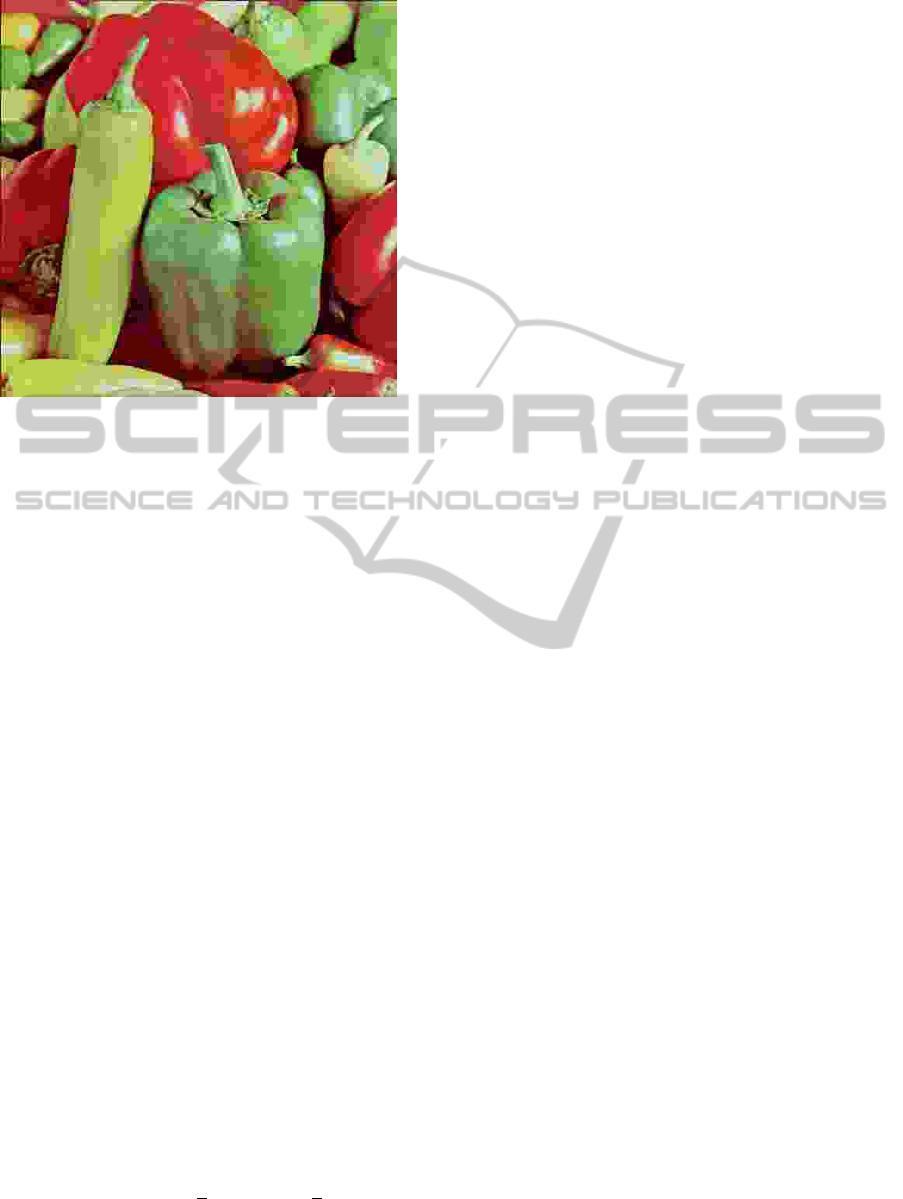
Figure 3: JPEG image with typical blocking and ringing
artifacts.
image, but a convex set of possible source images. In-
stead it just assumes the rounded integer value to be
the true quantized DCT coefficient which leads to the
well known JPEG artifacts as can be seen, for exam-
ple, in Figure 3.
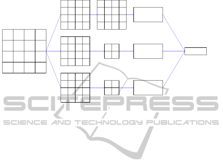
In the case of color images, typically a subsam-
pling of color components is performed as part of
JPEG compression. For that, color images are pro-
cessed in the YCbCr color space, i.e., the images are
given as u = (y,cb,cr), where y is the luminance com-
ponent and cb,cr are chroma components. Subsam-
pling is then applied to the chroma components cb
and cr, which reflects the fact that the human eye
is less sensitive to color variations than to bright-
ness variations. The resulting three image compo-
nents, which now differ in resolution, then undergo
the same process as grayscale images (see Figure
4). Again, the standard JPEG decompression simply
reverts this process, now by applying an additional
chroma-upsampling as last step.
An integral part of the model we propose is taking
the set of all possible source images associated with
a given JPEG object as a constraint. This set can be
mathematically described as follows. With the integer
coefficient data (d
c
i, j
), where the range of i, j depends
on the resolution of the color component c ∈{0, 1,2},
and the quantization matrix (Q
c
i, j
)
0≤i, j<8
, both pro-
vided by the compressed JPEG object, the set of num-
bers which yield d
c
i, j
in the quantization and rounding
step is given by the interval
J
c
i, j
=
Q
c
i, j
(d
c
i, j
−
1
2
),Q
c
i, j
(d
c
i, j
+
1
2
)
. (2)
Note that for this notation we extend the quantization
matrices up to the image dimensions simply by re-
peating the 8 ×8 coefficients. Having this, the coeffi-
cient data set D can be defined as
D =
(z
c
i, j
)|z
c
i, j
∈ J
c
i, j
for all c,i, j
(3)
and the set of possible source images of the compres-
sion process as
U
D
=
u = (u
c
i, j
)|ASu ∈D
(4)
where A is a color-component-wise blockwise DCT
operator and S is a subsampling operator (see Subsec-
tion 3.2 for the definition of A and S).
2.2 The TGV Functional
Another building block of the model is the total gen-
eralized variation functional (TGV) as proposed in
(Bredies et al., 2010), in particular of second order.
We give here a short definition and sum up some im-
portant results, for details and proofs however, we
refer to (Bredies et al., 2010; Bredies and Valko-
nen, 2011). The pre-dual formulation of second-order
TGV is given by
TGV
2
α
(u) = sup
(
Z
Ω
udiv
2
v dx
v ∈C
2
c
(Ω,S
2×2
),
kvk
∞
≤ α
0
,kdivvk
∞
≤ α
1
)
, (5)
where α = (α
0
,α
1
) ∈ R
2
, u ∈ L
1
(Ω) and S
2×2
is the
space of symmetric 2 by 2 matrices. Given a function
u ∈ L
1
(Ω), the second-order TGV functional takes
into account, as the test functions have the form div
2
v,
the generalized derivative of u up to order 2. Its kernel
is the set of polynomials with degree less than 2. Eval-
uation of TGV
2
α
can be also interpreted as an optimal
balancing of the first and second generalized deriva-
tive of u among themselves. This becomes obvious,
considering an equivalent representation of TGV
2
α
:
TGV
2
α
(u) = inf
v∈BD(Ω,R
d
)
α
1
k∇u −vk
1
+ α
0
kE (v)k
1
.
(6)
Here, E (v) denotes the symmetrized derivative of the
vector field v and BD(Ω) the space of vector fields
of bounded deformation. As one can also see in (6),
the ratio between the parameters α
1
and α
0
weights
the balancing between the first and second derivative
of u and will later also influence possible solutions of
TGV
2
α
regularized optimization problems. The TGV
functional possesses several properties which support
its usage as regularization term, such as convexity and
lower semi-continuity with respect to L
1
convergence.
It also satisfies a Poincar
´
e-Wirtinger type inequality
which can be used to obtain coercivitiy of the objec-
tive functional.
VISAPP 2012 - International Conference on Computer Vision Theory and Applications
14
YCbCr
8
42
246
90
100
7
230
86
78
226
56
165
Y
Cb
Cr
8
42
246
90
100
7
230
86
78
226
56
165
S
S
8
90
230 226
71
124
Grayscale-JPEG
Grayscale-JPEG
Grayscale-JPEG
Compressed image data
8 6 15 2 7 4 3 1
Figure 4: Chroma subsampling during JPEG compression.
3 THE METHOD
This section is devoted to present the TGV-based
JPEG reconstruction method. Let us at first state the
associated minimization problem in an infinite dimen-
sional setting. Note that we abuse notation by using
the same symbols for the continuous setting as for the
discrete one.
3.1 The Continuous Setting
For convenience we only consider grayscale images
for the continuous setting. Hence, our images are rep-
resented by real valued functions u ∈ L
2
(Ω) with Ω a
bounded Lipschitz domain, typically a rectangle. Us-
ing the definition of the TGV functional given in (5)
we can formulate the infinite dimensional minimiza-
tion problem as follows:
min
u∈L
2
(Ω)
TGV
2
α
(u) + I
U
D
(u) (7)
where
I
U
D
(u) =
(
0 if u ∈U
D
,
∞ else.
The data set U
D
can be defined as
U
D
= {u ∈ L
2
(Ω)|Au ∈ D}
where A is a basis transformation operator related to
a general orthonormal basis (a
n
)
n≥0
of L
2
(Ω). The
coefficient data set D ⊂`
2
reflects interval restrictions
on the coefficients:
D = {z ∈ `
2
|z
i
∈ J
i
∀i ∈ N
0
}
where J
i
⊂ R is a non-empty, closed (not necessarily
bounded) interval for any i ∈N
0
. Note that this model
allows arbitrary orthonormal bases (a
n
)
n≥0
of L
2
(Ω)
and constraints on infinitely many coefficients. How-
ever, for JPEG decompression, one usually chooses
an infinite block-cosine orthonormal basis, and lets
only the J
i
associated with the first 8 ×8 blockwise
coefficients be bounded and J
i
= R for the remaining
i, see (Bredies and Holler, 2011) for details.
Under assumptions which are satisfied in the ap-
plication of this model to JPEG decompression, we
can show existence of a solution to (7). More gen-
erally, if we assume that U
D
has non-empty interior
and that J
n
0
,J
n
1
,J
n
2
are bounded for certain n
0
,n
1
,n
2
,
existence of a solution can be guaranteed.
3.2 The Discrete Model
Based on the equivalent formulation of the TGV func-
tional in (6) and the data set U
D
as in (4) we will now
formulate our discrete model.
For k,l ∈ N, we set the space of discrete color im-
ages U = R
8k×8l×3
and further V = U
2
and W = U
3
.
The dimension 8k×8l ×3 results from the three color
components and reflects the fact that any JPEG image
is processed with its horizontal and vertical number
of pixels being multiples of 8.
Now for u ∈U, a discrete vector-input version of
the TGV
2
α
functional can be defined as
TGV
2
α
(u) = inf
v∈V
α
1
k∇(u) −vk
V
+ α
0
kE (v)k
W
, (8)
ARTIFACT-FREE JPEG DECOMPRESSION WITH TOTAL GENERALIZED VARIATION
15

where ∇ : U → V denotes a discrete, color-
component-wise gradient operator using forward dif-
ferences and E : V → W denotes a discrete, color-
component-wise symmetric gradient operator using
backward differences, i.e., E (v) =
1
2
(J(v) + J(v)
T
)
with J(v) a discrete color-component-wise Jacobian
of v. Note that in E (v), the off-diagonal entries
need to be stored only once, thus E(v) ∈ U
3
. For
v = (v
i, j
)
0≤i, j<8k
with v
i, j
∈ R
3×2
the norm on V is
defined as
kvk
V
:=
∑
i, j
|v
i, j
|
with |·| the Frobenius norm on R
3×2
. The norm k·k
W
is defined similarly.
In order to avoid extensive indexing, we will now
give just a local, component-wise definition of the op-
erators S and A, necessary to describe the data set U
D
.
The subsampling operator S depends on the foregoing
chroma subsampling process, but typically is defined
on disjoint 2 ×2 blocks of each chroma component,
denoted by (z
i, j
)
0≤i≤1
, as
Sz =
1
4
1
∑
m,n=0
z
m,n
,
reducing the resolution of the chroma components by
the factor 4. Since the resolution of the brightness
component is not reduced, S is the identity for this
component. The discrete cosine transformation op-
erator is defined, for each color component, on each
disjoint 8 ×8 block (z
i, j
)
0≤i, j≤7
, as
(Az)
p,q
= C
p
C
q
7
∑
n,m=0
z
n,m
cos
π(2n + 1)p
16
cos
π(2m + 1)q
16
,
for 0 ≤ p, q ≤ 7 and
C
s
=
(
1
√
8
if s = 0,
1
2
if 1 ≤ s ≤ 7.
With the operators S and A, the set U
D
can now be
defined as already done before in (4) by
U
D
= {u ∈U |ASu ∈ D},
where the coefficient data set D is obtained from the
compressed JPEG object as in (3).
With these prerequisites, the finite dimensional
optimization problem for artifact-free JPEG decom-
pression reads as
min
u∈U
TGV
2
α
(u) + I
U
D
(u), (9)
where again
I
U
D
(u) =
(
0 if u ∈U
D
,
∞ else.
Using the boundedness of the data intervals J
c
i, j
defined in (2) it can be shown that there exists a solu-
tion to (9) and that this problem is equivalent to
min
(u,v)∈U ×V
F(K(u, v)) + I
U
d
(u), (10)
where K : U ×V →V ×W,
K =
∇ −1
0 E
and F : V ×W → R,
F(v,w) = α
1
kvk
V
+ α
0
kwk
W
.
This formulation will now be the basis for the numer-
ical approach.
3.3 A Primal-dual Algorithm
We numerically solve our minimization problem us-
ing a primal-dual algorithm presented in (Chambolle
and Pock, 2011), for which convergence can be en-
sured. This algorithm is well-suited for this problem
because, as we will see, all necessary steps during one
iteration reduce to simple arithmetic operations and
the evaluation of a forward and inverse block-cosine
transformation, for which highly optimized code al-
ready exists. This makes the algorithm fast and also
easy to implement on the GPU.
As first step we note that (10) is equivalent to the
following saddle-point problem:
min
x∈X
max
y∈Y
((y,Kx)
Y,Y
−F
∗
(y) + I
U
D
(x)) (11)
where X = U ×V , Y = V ×W , (·,·) is the scalar
product on Y and F
∗
is the convex conjugate of F.
The primal-dual strategy for finding saddle points pre-
sented in (Chambolle and Pock, 2011) amounts to
performing the abstract iteration shown in Algorithm
1. Note that ∂F
∗
and ∂I
U
D
refers to the subdifferen-
tial of F
∗
and I
U
D
, respectively, and the operator K
∗
denotes the adjoint of K and is given by
K
∗
=
−div 0
−1 −div
2
with div = −∇
∗
and div
2
= −E
∗
denoting discrete
divergence operators.
Using standard arguments from convex analysis,
it can be shown that the resolvent-type operators (I +
σ ∂ F
∗
)
−1
and (I +τ ∂ I
U
D
)
−1
take the following form:
(I + σ∂F
∗
)
−1
(v, w) =
proj
α
1
(v),proj
α
0
(w)
VISAPP 2012 - International Conference on Computer Vision Theory and Applications
16

where
proj
α
1
(v) =
v
max(1,
kvk
∞
α
1
)
,
proj
α
0
(w) =
w
max(1,
kwk
∞
α
0
)
and
(I + τ ∂I
U
D
)
−1
(u,v) =
u + S
−1
proj
U
A
(Su) −Su
,v
where
proj
U
A
(u) = A
∗
z
with
z
c
i, j
=
u
c
i, j
if (Au)
c
i, j
∈ J
c
i, j
= [l
c
i, j
,r
c
i, j
]
r
c
i, j
if (Au)
c
i, j
> r
c
i, j
l
c
i, j
if (Au)
c
i, j
< l
c
i, j
,
A
∗
= A
−1
the adjoint of A and S
−1
denoting the up-
sampling operator associated with S, given locally by
replication of z ∈ R, i.e.,
S
−1
z =
z z
z z
.
Having this, we can now give the concrete imple-
mentation of the primal-dual algorithm for JPEG de-
compression in Algorithm 2. Note that the step-size
restriction στ ≤
1
12
results from the estimate kKk
2
<
12. As one can see, all steps of Algorithm 2 can
be evaluated by simple, mostly pixel-wise operations
making each iteration step fast.
4 NUMERICAL EXPERIMENTS
We implemented and tested the proposed TGV-based
JPEG decompression method. First of all, we have
compared the standard JPEG decompression with our
method for three images possessing different charac-
teristics. The outcome can bee seen in Figure 5, where
also the image dimensions and the memory require-
ment of the JPEG compressed image is given in bits
Algorithm 1: Abstract primal-dual algorithm.
• Initialization: Choose τ,σ > 0 such that
kKk
2
τσ < 1, (x
0
,y
0
) ∈ X ×Y and set x
0
= x
0
• Iterations (n ≥0): Update x
n
,y
n
,x
n
as follows:
y
n+1
= (I + σ ∂ F
∗
)
−1
(y
n
+ σKx
n
)
x
n+1
= (I + τ ∂I
U
D
)
−1
(x
n
−τK
∗
y
n+1
)
x
n+1
= 2x
n+1
−x
n
per pixel (bpp). As one can see, our method performs
well in reducing the typical JPEG artifacts and still
preserves sharp edges.
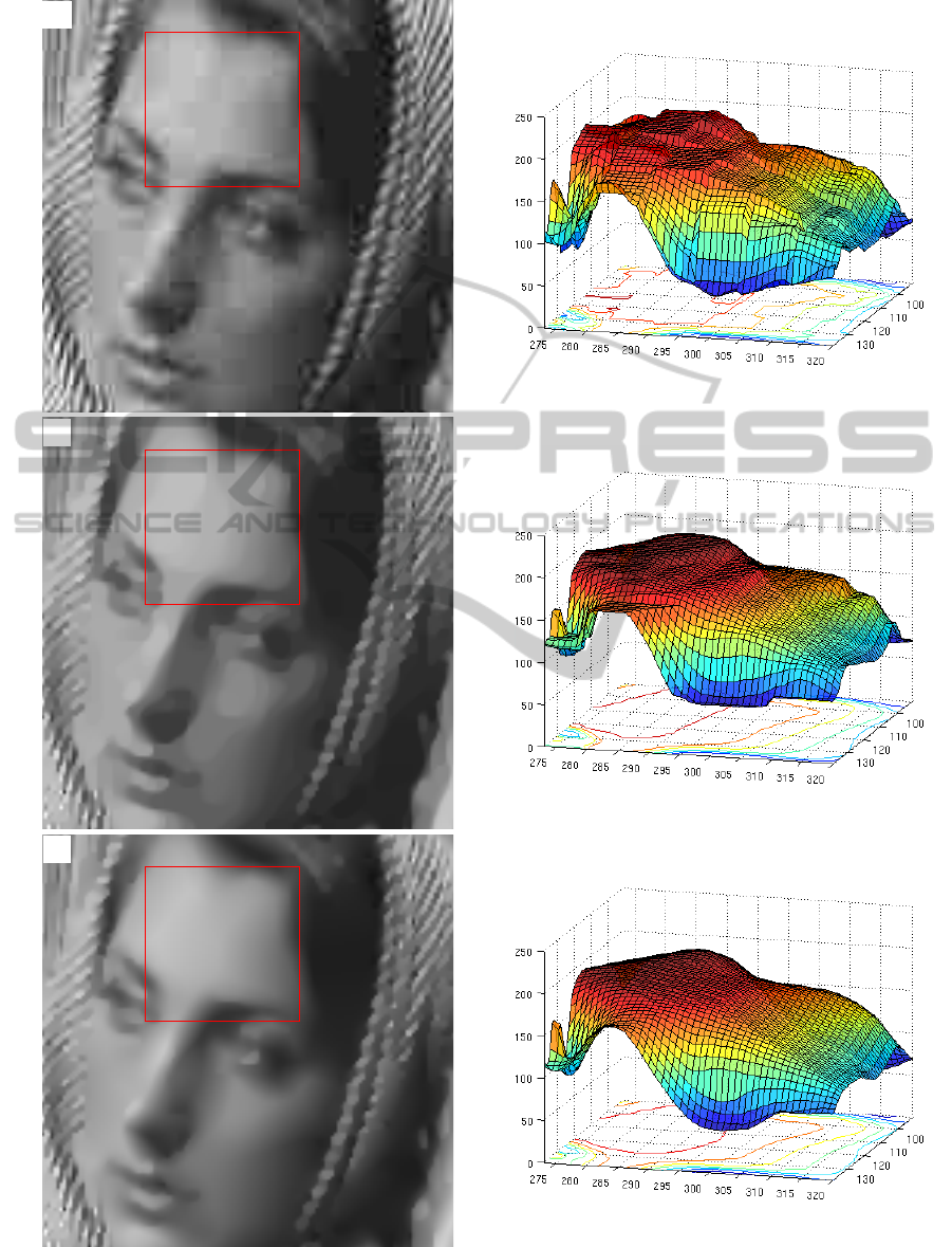
Figure 6 then allows to compare our results with
the reconstruction using TV instead of TGV as reg-
ularization functional as proposed in (Bredies and
Holler, 2011). As one can see, in particular in the sur-
face plots, the TV-based method also maintains sharp
edges. However, it leads to a staircasing effect in re-
gions that should be smooth. In contrast to that, the
TGV-based method yields a more natural and visually
more appealing reconstruction in such regions.
Figure 7 serves as an example of an image con-
taining texture. It can be seen that our method pre-
serves fine details and does not lead to additional
smoothing of textured regions.
We also developed a parallel implementation of
the method for multi-core CPUs and GPUs, us-
ing OpenMP (OpenMP Architecture Review Board,
2011) and Nvidia’s Cuda (NVIDIA, 2008), respec-
tively. For the GPU implementation we partly used
kernel functions adapted to the compute capability of
the device. The blockwise DCT was performed on
the CPU and the GPU using FFTW (Frigo and John-
son, 2005) and a block-DCT kernel provided by the
Cuda SDK, respectively. Computation times of those
implementations for multiple image sizes are given in
Table 1. As one can see, especially the GPU imple-
mentation yields a high acceleration and makes the
method suitable for real-time applications. The given
Algorithm 2: Scheme of implementation.
1: function TGV-JPEG(J
comp
)
2: (d,Q) ← Decoding of JPEG-Object J
comp
3: d ← d ·Q
4: u ←S
−1
(A
∗
(d))
5: v ←0,u ←u,v ←0, p ←0,q ←0
6: choose σ,τ > 0 such that στ ≤1/12
7: repeat
8: p ← proj
α
1
(p + σ(∇u −v))
9: q ← proj
α
0
(q + σ(E (v))
10: u
+
← u + τ(div p)
11: v
+
← v + τ(p + div
2
q)
12: u
+
← u
+
+ S
−1
(proj
U
A
(Su
+
) −Su
+
)
13: u ← (2u
+
−u), v ← (2v
+
−v)
14: u ← u
+
, v ← v
+
15: until Stopping criterion fulfilled
16: return u
+
17: end function
ARTIFACT-FREE JPEG DECOMPRESSION WITH TOTAL GENERALIZED VARIATION
17
A B
C D
E F
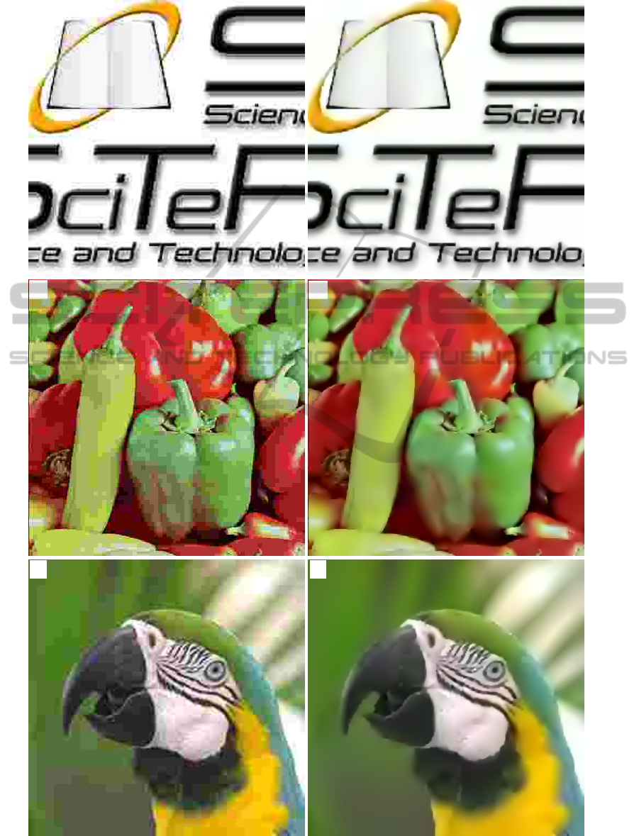
Figure 5: On the left: Standard decompression, on the right: TGV-based reconstruction after 1000 iterations. A-B: SciTePress
image at 0.5 bpp (256 ×256 pixels). C-D: Peppers image at 0.15 bpp (512 ×512 pixels). E-F: Parrot image at 0.3 bpp
(256 ×256 pixels).
VISAPP 2012 - International Conference on Computer Vision Theory and Applications
18
A
B
C
Figure 6: Close-up of Barbara image at 0.4 bpp at 1000 iterations. The marked region on the left is plotted as surface on the
right. A: Standard decompression. B: TV-based reconstruction. C: TGV-based reconstruction.
ARTIFACT-FREE JPEG DECOMPRESSION WITH TOTAL GENERALIZED VARIATION
19
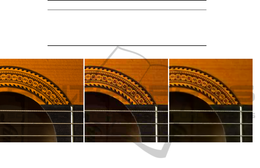
Table 1: Computation times in seconds to perform 1000 iterations for different devices and image sizes. CPU: AMD Phenom
9950. GPUs: Nvidia Quadro FX 3700 (compute capability 1.1), Nvidia GTX 280 (compute capability 1.3), Nvidia GTX 580
(compute capability 2.0). Note that on the Quadro FX 3700 and GTX 280, not enough memory was available to perform the
algorithm for the 3200 ×2400 pixel image.
Device 512 ×512 1600 ×1200 3200 ×2400
CPU Single-core 53.22 672.51 1613.44
CPU Quad-core 28.32 263.70 812.18
GPU Quadro FX 3700 4.92 35.52 -
GPU Nvidia GTX 280 2.2 10.22 -
GPU Nvidia GTX 580 1.2 6.6 25.70
Figure 7: From left to right: Uncompressed image at 24 bpp (256 ×256 pixels), standard decompression of JPEG com-
pressed image at 1.06 bpp, TGV-based reconstruction of the same JPEG compressed image after 1000 iterations. Image by
(Dawgbyte77, 2008), licensed under CC-BY-2.0 (http://creativecommons.org/licenses/by/2.0/).
computation times correspond to the computation of
1000 iterations, which is in most cases more than
enough for a reconstruction visually almost indistin-
guishable from one obtained as optimal solution satis-
fying a suitable stopping criterion. Since the decrease
of the TGV-value of the image is typically very high
especially during the first iterations of the algorithm,
and since a fit-to-data can be ensured for any iteration
step image, one could use the image obtained after
only a few number of iterations as intermediate re-
construction and then iteratively update the solution.
5 SUMMARY AND
CONCLUSIONS
We proposed a novel method for the improved recon-
struction of given JPEG compressed images, in partic-
ular, color images. The reconstruction is performed
by solving a non-smooth constrained optimization
problem where exact data fidelity is achieved by the
usage of a convex indicator functional. The main nov-
elty, however, lies in the utilization of TGV of sec-
ond order as a regularization term which intrinsically
prefers natural-looking images, as it has been con-
firmed in Section 4. This was shown to be true not
only with respect to the standard reconstruction, but
also with respect to already-known TV-based recon-
struction methods.
Moreover, a parallel implementation for multi-
core CPUs and GPUs showed that this reconstruction
process can be realized sufficiently fast in order to
make the method also applicable in practice.
Motivated by these promising results, the focus of
further research will be the development of a theory
for a more general model using the TGV functional
of arbitrary order.
ACKNOWLEDGEMENTS
Support by the Austrian Science Fund FWF under
grant SFB F032 (“Mathematical Optimization and
Applications in Biomedical Sciences”) is gratefully
acknowledged.
VISAPP 2012 - International Conference on Computer Vision Theory and Applications
20

REFERENCES
Alter, F., Durand, S., and Froment, J. (2005). Adapted to-
tal variation for artifact free decompression of JPEG
images. Journal of Mathematical Imaging and Vision,
23:199–211.
Bredies, K. and Holler, M. (2011). A total-variation-
based JPEG decompression model. Submitted
for publication. Preprint available at http://math.uni-
graz.at/mobis/publications.html.
Bredies, K., Kunisch, K., and Pock, T. (2010). Total gener-
alized variation. SIAM Journal on Imaging Sciences,
3(3):492–526.
Bredies, K. and Valkonen, T. (2011). Inverse problems with
second-order total generalized variation constraints.
In Proceedings of SampTA.
Caselles, V., Chambolle, A., and Novaga, M. (2007). The
discontinuity set of solutions of the TV denoising
problem and some extensions. Multiscale Model.
Simul., 6:879–894.
Chambolle, A. and Pock, T. (2011). A first-order primal-
dual algorithm for convex problems with applications
to imaging. Journal of Mathematical Imaging and Vi-
sion, 40:120–145.
Dawgbyte77 (2008). http://www.flickr.com/photos/dawg-
byte77/3052164481/.
Frigo, M. and Johnson, S. G. (2005). The design and im-
plementation of FFTW3. Proceedings of the IEEE,
93(2):216–231. Special issue on “Program Genera-
tion, Optimization, and Platform Adaptation”.
Kartalov, T., Ivanovski, Z. A., Panovski, L., and Karam,
L. J. (2007). An adaptive POCS algorithm for com-
pression artifacts removal. In 9th International Sym-
posium on Signal Processing and Its Applications,
pages 1–4.
Nikolova, M. (2000). Local strong homogeneity of a regu-
larized estimator. SIAM J. Appl. Math., 61:633–658.
Nosratinia, A. (2001). Enhancement of JPEG-compressed
images by re-application of JPEG. The Journal of
VLSI Signal Processing, 27:69–79.
NVIDIA (2008). NVIDIA CUDA programming guide 2.0.
NVIDIA Cooperation.
OpenMP Architecture Review Board (2011). Openmp
application program interface, version 3.1.
http://www.openmp.org.
Ring, W. (2000). Structural properties of solutions to to-
tal variation regularization problems. M2AN Math.
Model. Numer. Anal., 34:799–810.
Shen, M.-Y. and Kuo, C.-C. J. (1998). Review of postpro-
cessing techniques for compression artifact removal.
Journal of Visual Communication and Image Repre-
sentation, 9(1):2–14.
Singh, S., Kumar, V., and Verma, H. K. (2007). Reduc-
tion of blocking artifacts in JPEG compressed images.
Digital Signal Processing, 17(1):225–243.
Wallace, G. K. (1991). The JPEG still picture compression
standard. Commun. ACM, 34(4):30–44.
Weerasinghe, C., Liew, A. W.-C., and Yan, H. (2002). Arti-
fact reduction in compressed images based on region
homogeneity constraints using the projection onto
convex sets algorithm. IEEE Transactions on Circuits
and Systems for Video Technology, 12(10):891–897.
Zhong, S. (1997). Image coding with optimal reconstruc-
tion. In International Conference on Image Process-
ing, volume 1, pages 161–164.
Zou, J. J. and Yan, H. (2005). A deblocking method for
BDCT compressed images based on adaptive projec-
tions. IEEE Transactions on Circuits and Systems for
Video Technology, 15(3):430–435.
ARTIFACT-FREE JPEG DECOMPRESSION WITH TOTAL GENERALIZED VARIATION
21
