EXTRACTION OF REGION BOUNDARY PATTERNS
WITH ACTIVE CONTOURS
Mohamed Ben Salah
1
and Amar Mitiche
2
1
Department of Computing Science, University of Alberta, Edmonton, AB, Canada
2
Institut National de la Recherche Scientifique, Montreal, QC, Canada
Keywords:
Image Segmentation, Boundary Features, Distributions Matching, Active Curves, Level Sets.
Abstract:
In this study we address the problem of recovering region boundary patterns consistent with a given pattern. A
level set method formulated in the variational framework evolves an active contour towards regions of interest
boundaries while omitting the others. The curve evolution results from the minimization of a functional which
measures the similarity between the distribution of an image-based geometric feature on the curve and a
model distribution. The corresponding curve evolution equation can be viewed as a geodesic active contour
flow having a variable stopping function. This affords a global representation of the objects boundaries which
can effectively drive active curve segmentation in a variety of otherwise adverse conditions. We ran several
experiments supported by quantitative performance evaluations using various examples of segmentation and
tracking.
1 INTRODUCTION
Image segmentation is a central problem and ex-
tensively researched topic in computer vision. It
serves numerous applications such as medical image
analysis, robotics, surveillance, and remote sensing
(Holtzman-Gazit et al., 2006; Ben Ayed et al., 2005;
Mortensen, 2008).
Leading to the most effective, numerically effi-
cient and stable algorithms, the active contour varia-
tional formulations are widely adopted in a variety of
settings (Chan and Vese, 2001; Cremers et al., 2007;
Freedman and Zhang, 2004; Ben Ayed et al., 2009;
Paragios and Deriche, 2002). The problem is formu-
lated as a minimization problem of an objective func-
tional which embeds the constraints on the segmen-
tation. The ensuing Euler-Lagrange equations, min-
imizing the objective functional, are evolution equa-
tions which drive the active contours towards the rele-
vant region boundaries. The objective functional data
terms, which measure the conformity of the image to
model descriptions, are either edge-based when they
evaluate an image function along the active curve, or
region-based when they refer to the image within the
region enclosed by the curve. Therefore, the corre-
sponding curve evolution velocities are due to the im-
age exclusively along or within the curve.
Edge-based methods have been among the first ac-
tive contour solutions proposed for image segmenta-
tion problems. The Snake model (Kass et al., 1988),
and the geodesic active contour (GAC) which adopted
a more effective curve representation (Caselles et al.,
1997), were precursory of a vast literature on edge-
based active curve image segmentation (Kass et al.,
1988; Caselles et al., 1997; Paragios et al., 2004;
Kichenassamy et al., 1995; Paragios and Deriche,
2002). Typically, these algorithms attract the active
curve toward high contrast boundaries of the image,
which are assumed to coincide with desired regions
boundaries, by minimizing a geodesic integral along
the contour of a decreasing function of the image
gradient. In general, geodesics are seriously chal-
lenged when the desired boundaries have segments
of low gradient or when all the objects, the desired
and non desired objects, present high image transi-
tions ans similar intensity profiles. For instance, in
magnetic resonance imaging (MRI) and computed to-
mography (CT) medical images, the organs of interest
can present very weak edges and high intensity simi-
larity with neighboring structures. In such cases, the
geodesic contours leak away from the desired bound-
aries and may vanish.
Region-based schemes, which refer to the image
over regions, were later proposed to overcome these
kind of problems. In region-based algorithms, each
segmentation region is characterized by an image dis-
240
Ben Salah M. and Mitiche A..
EXTRACTION OF REGION BOUNDARY PATTERNS WITH ACTIVE CONTOURS.
DOI: 10.5220/0003826102400248
In Proceedings of the International Conference on Computer Vision Theory and Applications (VISAPP-2012), pages 240-248
ISBN: 978-989-8565-03-7
Copyright
c
 2012 SCITEPRESS (Science and Technology Publications, Lda.)

tribution, i.e., the regions are assumed to differ by
their image statistics. Hence, they are significantly
less sensitive to weak boundary gradient than the
geodesic schemes (Chan and Vese, 2001; Zhu and
Yuille, 1996; Samson et al., 2000; Ben Ayed et al.,
2005). Following the seminal work of Chan and Vese
(Chan and Vese, 2001) which uses region means, var-
ious algorithms have been proposed. In general, they
use a global model description of the image within
the extent of each desired region to penalize move-
ments of the active curves in or out of the regions
they are intended to delineate. Both parametric (Chan
and Vese, 2001; Mansouri et al., 2006; Ben Ayed
et al., 2006; Salah et al., 2010) and non-parametric
(Freedman and Zhang, 2004; Rousson and Cremers,
2005; Michailovich et al., 2007) image descriptions
have been used for the purpose. However, and in
spite of this accrued robustness, the region-based ac-
tive curve evolution can be seriously challenged, by
definition, when the regions to segment have similarly
distributed segments (Ben Ayed et al., 2009). When
these segments occur between regions, the placement
of the separating boundary becomes largely ambigu-
ous.
Other methods combine the advantages of both
edge-based and region-based models in order to over-
come the mentioned problems (Paragios and Deriche,
2002; Vazquez et al., 2006). However, current meth-
ods are still not applicable especially when the tar-
get regions are rather characterized by the distribu-
tion of a feature on their boundary. In other words,
this happens when region boundaries are considered
patterns described by a geometric feature distribution
rather than simply the location of the feature as with
typical geodesic descriptions. One typical example
where this description of boundaries by a geometric
feature distribution is befitting is depicted in Figure 1.
This example is of an image where regions occur with
boundaries that are either rectangular or ellipsoidal
outline. For each outline pattern there are two regions
of varying appearance and the goal of segmentation
is to extract, in a single instantiation, the regions of
each of the two patterns. Matching the distribution of
boundary curvature, measured from the image gra-
dient, against a model distribution, has extracted both
rectangular regions in one case (Figure 1 (a)) and both
ellipsoidal regions in the other (Figure 1 (b)), without
prior knowledge of the number of regions. Note that
a shape prior constraint will not be able to segment
all of the regions of the same figure, unless one such
prior is used for each region, and each with an accom-
panying close by initialization, which supposes an in-
formation about the image not available for practical
purposes, such as the number of objects as well as the
(a) (b)
Figure 1: The segmentation targets elliptical objects in (a)
and rectangular objects in (b). Only the targeted objects
should be segmented.
section of the image domain where each occurs (Cre-
mers et al., 2003; Chan and Zhu, 2005). Because, a
shape prior is an image-independentterm added to the
segmentation functional so as to bias a detected region
to have a given geometric outline modulo a transfor-
mation (such as rigid or affine) (Cremers et al., 2007;
Leventon et al., 2000; Cremers et al., 2006), a shape
prior constraint will also require additional optimiza-
tion over pose transformations, or a constraint on the
curve deformation with respect to a reference shape
(Foulonneau et al., 2006; Foulonneau et al., 2009).
The purpose of this study is to take full advan-
tage of the statistical image information that one can
learn about the boundary of interest. We investigate
a level set variational segmentation method which
drives an active curve to coincide with boundaries on
which a geometric feature distribution matches a ref-
erence distribution. Indeed, we propose to minimize
a contour-based functional which measures the simi-
larity between the distribution of an image-based ge-
ometric feature along the curve and a reference dis-
tribution learned a priori. The scheme is formulated
using the Kullback-Leibler similarity measure and is
applied to simultaneously recover all region bound-
aries consistent with a given outline pattern using the
isophote curvature as the geometric feature. Note that
other features can be used such as the differences of
curvatures and angle tangents, and also other simi-
larity measures such as the Bhattacharyya measure
can be adopted. A detailed experimentation (Sec-
tion 4) shows that the scheme is valid and can im-
prove on region and edge based methods. Compared
to the region-based formulations in (Freedman and
Zhang, 2004; Ben Ayed et al., 2009; Michailovich
et al., 2007), the objectives of the proposed function-
als are fundamentally different. For instance, the for-
mulations in (Freedman and Zhang, 2004; Ben Ayed
et al., 2009; Michailovich et al., 2007) would not dis-
tinguish, and it is not their purpose, between the el-
liptical and rectangular regions in Figure 1 (a,b) be-
cause these regions have exactly the same image dis-
tributions. The marginal similarity with these studies
is in using global measures, but the curve evolution
EXTRACTION OF REGION BOUNDARY PATTERNS WITH ACTIVE CONTOURS
241

equations we obtained are quite different. Such a dif-
ference will be evidenced in the experiments. Min-
imization of the proposed functional is carried out
by deriving Euler-Lagrange equations implemented
via level set techniques. Interestingly, each of the
evolution equations we obtained can be viewed as a
GAC having a variable stopping function. However,
the stopping functions have two fundamental differ-
ences with the usual GAC stopping function. First,
they depend both on the image and the curve, when
the GAC stopping function depends only on the im-
age. Second, they reference the curvature distribu-
tion along the contour, a global information, rather
than just pixel-wise characteristic as with GAC; such
a richer information should afford a better boundary
detection behavior. An interpretation of this behavior
will be discussed later.
2 FORMULATION
2.1 Objective Function
Let I : Ω ⊂ R
2
→ R be an image function, γ : [0,1] →
Ω a simple closed plane parametric curve, and F : Ω ⊂
R
2
→ F ⊂ R a feature function from the image do-
main Ω to a feature space F . Let P
γ
be a kernel den-
sity estimate of the distribution of F along γ,
∀f ∈ F P
γ
( f) =
H
γ
K( f −F
γ
)ds
L
γ
, (1)
where F
γ
is the restriction of F to γ, L
γ
is the length of
γ given by L
γ
=
H
γ
ds, and K is the estimation kernel.
In this work, we consider the Gaussian kernel of width
h given by
K(z) =
1
√
2πh
2
exp
−
z
2
2h
2
. (2)
Given a model feature distribution M , let
D(P
γ
,M ) be a similarity measure between P
γ
and M .
The purpose of this work is to determine
˜
γ such that
˜
γ = argmin
γ
D(P
γ
,M ). (3)
To apply this formulation we need to specify the
feature function, the model, the similarity, and a
scheme to conduct the objective functional minimiza-
tion in Eq. (3).
2.2 Feature
Various types of image-base features can be em-
ployed depending on the segmentation problem at
hand. There are two fundamental types of boundary
representation features. One type is the photometric,
where the feature is a function of the image such as
image intensity, its gradient, or any scalar image fil-
ter output. The other type of feature function is the
geometric, which pertains to the boundary form, irre-
spective of the image function. The curvature, which
belongs to this category, is the feature adopted in this
work. It can be estimated from the image under the
assumption that the region boundary normals coin-
cide with the isophote normals:
F = κ
I
= div

∇I
k∇Ik

. (4)
Studies have shown that curvature histograms,
which can be viewed as empirical marginal distri-
butions of the shape considered a random variable,
are useful statistics to describe closed regular plane
shapes (Zhu, 2003). Ideally, a geometric descrip-
tion is invariant to the shape position, orientation, and
size. It must also be robust to the distortions which
normally affect the shape. Curvature, which is the
rate of change of the tangent angle along the contour
(Do Carmo, 1976), is invariant to translation and rota-
tion but varies with scale. However, this variability is
taken into account by an affine transformation of the
curvature values so that they always correspond to the
same set of bins. For practical means, this normaliza-
tion makes the histograms unaffected by scale.
Geometric features are necessary when the tar-
get object boundary has no specific photometric de-
scription, either because the description varies with
the picture in which the object appears (e.g., as in
Fig. 4 where objects can appear with different col-
ors/textures and/or over different backgrounds) or be-
cause there are no photometric features which would
distinguish the target from other objects in the image
(as in Fig. 2).
2.3 Similarity
The Kullback-Leibler divergence is a common simi-
larity function between distributions. Several studies
have used it for foreground-background image seg-
mentation (Mitiche and Ayed, 2010). Efficient ap-
plications of the Kullback-Leibler divergence have
been reported in (Freedman and Zhang, 2004) in ac-
tive contour segmentation. It has been part of effec-
tive image segmentation formulations (Freedman and
Zhang, 2004) (Mansouri and Mitiche, 2002) (Myro-
nenko and Song, 2009) (Lecellier et al., 2009). As
well, the bhattacharyya coefficient has also been im-
plemented to match the distribution along contours
of a local image average to the distribution along a
model object boundary (Ben Ayed et al., 2010). Stud-
VISAPP 2012 - International Conference on Computer Vision Theory and Applications
242

ies which mention or use both measures have pre-
sented them as alternatives.
We implemented the minimization in Eq. 3 for the
Kullback-Leibler divergence as the similarity func-
tion D. The Kullback-Leibler divergence between P
γ
and M is
D(P
γ
,M ) = KL(P
γ
,M ) =
Z
F
M ( f) log
M ( f)
P
γ
( f)
d f.
(5)
Higher values of the Kullback-Leibler divergence
indicate smaller overlaps between the distributions.
The symmetry of the similarity function with re-
spect to its two distribution arguments (the Kullback-
Leibler divergence is not symmetric) is not an issue
here because we want to asses how close a variable
distribution is to a fixed (model) distribution. Next,
we derive the Euler-Lagrange descent equations cor-
responding to Eq. (3) for the Kullback-Leibler simi-
larity.
3 MINIMIZATION
The data term in Eq. (3) is a measure of similarity
between distributions over the boundary representa-
tion curve γ. We will address this problem by contin-
uous optimization via the associated Euler-Lagrange
γ-evolution descent equations. Let γ be embedded in a
one-parameter family of curves indexed by (algorith-
mic) time t:γ(s,t) : [0,1] ×R
+
→ Ω, and deriving the
Euler-Lagrange descent equation
∂γ
∂t
= −
∂D
∂γ
. (6)
For D(P
γ
,M ) = KL(P
γ
,M ), we have:
∂D
∂γ
=
∂KL
∂γ
=
Z
F
M ( f)
∂
∂γ
log

M ( f)
P
γ
( f)

d f
= −
Z
F
M ( f)
∂
∂γ
log

H
γ
K( f −F
γ(s)
)ds
L
γ

d f
=
∂L
γ
L
γ
∂γ
−
Z
F
M ( f)
∂
∂γ
log

I
γ
K( f −F
γ(s)
)ds

d f
(7)
where, we recall, F
γ
is the restriction of F to γ. Both
curve length L
γ
and the second integral in Eq. 7 can
be written as
H
γ
hds, where h is a scalar function, and
their functional derivative with respect to γ is of the
form (Caselles et al., 1997):
∂
H
γ
hds
∂γ
= (−hκ + ∇h·~n)~n, (8)
where~n is the inward unit normal to γ and κ its mean
curvature function. Therefore,
∂
∂γ
log

I
γ
K( f −F
γ(s)
)ds

=
∂
∂γ
H
γ
K( f −F
γ(s)
)ds
H
γ
K( f −F
γ(s)
)ds
=
−K( f −F
γ
)κ+ ∇K( f −F
γ
) ·~n
H
γ
K( f −F
γ(s)
)ds
~n (9)
and
∂L
γ
∂γ
= −κ~n.
This gives
∂γ
∂t
=
κ
L
γ
~n−
h
κ
L
γ
Z
F
M ( f)
P
γ
( f)
K( f −F
γ
)d f
i
~n
+
~n
L
γ
∇

Z
F
M ( f)
P
γ
( f)
K( f −F
γ
)d f

·~n
=
1
L
γ
h
1−
Z
F
M ( f)
P
γ
( f)
K( f −F
γ
)d f

κ
|
{z }
Stopping f orce
+∇

Z
F
M ( f)
P
γ
( f)
K( f −F
γ
)d f

·~n
|
{z }
Refinement force
i
~n (10)
which can be written as:
∂γ
∂t
=



G
KL
(P
γ
,M , F
γ
)κ
|
{z }
Stopping
−∇G
KL
(P
γ
,M , F
γ
) ·~n
|
{z }
refinement



~n.
(11)
The evolution equation (11) is of an ordinary geodesic
active contour form (Caselles et al., 1997) except that
the function G
KL
is variable since it depends on the
evolving contour, and it references a global informa-
tion. In general, global information affords added
strength to local descriptions in order to ensure sta-
ble curve evolution.
When the curve is close to the desired boundary,
close to adhering, the curve has a feature density close
to the reference density, i.e., P(F
γ(p)
) ≈ M(F
γ(p)
),
which implies that G
KL
≈ 0. Consequently, the curve
behavior is predominantly modulated by the gradient
term which drives it to adhere to the desired bound-
ary because it constrains it to move so as to coincide
with local highs in the model and curve distributions
similarity, just as the common GAC gradient term
guides the curve toward local highs in image contrast
(Caselles et al., 1997).
3.1 Level Set Implementation
The curve evolution equation is implemented using
level set method. The active curve γ(s,t) is implicitly
EXTRACTION OF REGION BOUNDARY PATTERNS WITH ACTIVE CONTOURS
243

represented by the zero level of a function φ(x,t) :
Ω ×R
+
→ R, i.e., γ = {x ∈ Ω | φ(x,t) = 0}. Recall
(Sethian, 1999) that when γ evolves according to
∂γ(s,t)
∂t
= V(s,t)~n(s,t), (12)
then φ evolves according to
∀x ∈Ω,
∂φ(x,t)
∂t
= V(x,t)k∇φ(x,t)k, (13)
with the conventionthat φ > 0 inside the zero level-set
and ~n is oriented inward. Hence, the level set evolu-
tion equation corresponding to the flow (11) is given
by
V(x,t) = G(P
φ
,M , F) κ
φ
−∇G(P
φ
,M , F)·
∇φ(x,t)
k∇φ(x,t)k
(14)
where G is G
KL
. The stopping function is variable of
the curve and, therefore, must be updated during evo-
lution using the sample feature distribution within a
narrow band δ around the zero level set of φ (Sethian,
1999):
P
φ
( f) =
R
−δ<φ(x)<δ
K( f −F(x))dx
R
−δ<φ(x)<δ
dx
. (15)
κ
φ
is the mean curvature function of φ:
κ
φ
(x,t) = div

∇φ(x,t)
k∇φ(x,t)k

, ∀x ∈Ω (16)
Geodesic evolution is often quickened by an ad-
ditional constant speed c along the curve normal
(Caselles et al., 1997), resulting in the level set mo-
tion (Li et al., 2005)
∂φ(x,t)
∂t
= (V(x,t) + c)k∇φ(x,t)k (17)
4 EXPERIMENTS
In this section we apply the proposed method to var-
ious experiments illustrating different applications in
order to demonstrate its stated advantages. Indeed,
the purpose of this set of experiments is to show that
the method can effectively extract, in a single instan-
tiation, all of the regions in an image whose (geomet-
ric) feature boundary distribution follows a learned
outline pattern. The examples include evaluations
over color images from the ETHZ database (Ferrari
et al., 2006; Ferrari et al., 2009) and over medical im-
ages.
In this set of experiments, we compared the pro-
posed matching functional (abbreviated CDM here-
after) to the following functionals:
(a) (b) (c) (d)
Figure 2: Detection of regions whose boundaries are consis-
tent with learned outline patterns. Each row depicts a seg-
mentation of the image corresponding to a different model
of curvature learned a priori. For example, for the first row
the model of curvature is learned independently from the
shape of a single rectangle; and for the second row it is
learned from a single ellipse with approximately the same
aspect ratio as in the figure. Columns: (a) Initial curve posi-
tions,(b) training images and contours, (c) the final segmen-
tations, and (d) segmentation with the GAC model (upper)
and the RL piece-wise constant model (lower).
RL: The region-based likelihood functional com-
monly used in image segmentation (Chan and Vese,
2001; Paragios and Deriche, 2002; Rousson and Cre-
mers, 2005; Boykov and Funka Lea, 2006). Opti-
mization of this functional seeks a two-region parti-
tion maximizing the conditional probability of pixel
data given the learned models within the segmenta-
tion regions.
GAC: The classical geodesic active contour func-
tional (Caselles et al., 1997) commonly used in image
segmentation as an edge-based constraint, which bi-
ases the segmentation boundaries towards high gradi-
ents of image data.
GAC-SP: Concatenation of GAC with a shape prior
term.
In all the experiments, the feature distribution is
estimated using the kernel width h= 1 and the narrow
band parameter δ = 1.
As stated before, the purpose here is to recover
region boundaries consistent with an outline pattern
without prior knowledge of the number of regions.
Intensity based methods would not allow to do this
because, as illustrated in the simple synthetic image
of Fig. 2, the targeted regions may have the same
intensity distribution as unwanted differently shaped
regions. Instead, we will use a geometric feature,
namely curvature. Using curvature affords a scheme
which handles differences in the pose and number of
targeted regions. This is in sharp contrast with shape
prior methods which require the knowledge of the
number of regions and inclusion of pose parameters
in the optimization.
Synthetic Example: Fig. 2 is a synthetic image of
VISAPP 2012 - International Conference on Computer Vision Theory and Applications
244

a row of three ellipses of appearances but with ap-
proximately the same aspect ratio and a row of dif-
ferent rectangles. The purpose is to segment either
all of the rectangular regions, in one instantiation, or
all of the ellipsoidal regions but not both. The model
curvature (Eq. 4) distributions are learned from one
rectangle and one ellipse independently from those
appearing in Fig. 2. The contour evolves first towards
high contrast boundaries. Once the region boundaries
are reached, the proposed CDM flow causes the ac-
tive curve to remain in coincidence with the desired
boundaries but leaves and vanishes from the others.
For example, along the boundary of the rectangles
(second row), the feature distribution does not match
the model distribution of curvature along an ellipse.
Therefore, the contour continues to evolve inside the
rectangles, and delineates only the elliptical regions
at convergence. Evidently, neither region-based seg-
mentation (via RL, for instance) nor edge-based seg-
mentation (via GAC, for instance) will be able to dis-
tinguish one type of regions from the other (last col-
umn of Fig. 2).
Real Example: The purpose of the second experi-
ment (cf. Fig. 3) is to show the advantage over stan-
dard algorithms such as GAC in the case of multiple
occurrences of the desired object in a real image. Fig.
3 depicts an example of segmentation of vertebrae in a
CT scan of the human spine. The distribution of cur-
vature has been approximated by a histogram along
the outline of an exemplar vertebra. Although the re-
sults are not totally accurate, CDM (Fig. 3(a)) has
been able to segment correctly two vertebrae, do a de-
cent outlining of the others (the poor segmentation of
the upper vertebra is due to border effects as no ini-
tialization could include this vertebra), and ignore the
bone structures on the right. Of course, region-based
methods cannot handle this example because the im-
age profile within the vertebrae is very similar to that
of other surrounding structures. Edge-based function-
als, such as GAC, will bias the active contour to all
high image gradients which do not correspond neces-
sarily to the edges of the vertebrae. GAC (Fig. 3(b))
has not been able to do as well on the vertebrae and
has included the bone structures on the right.
ETHZ Dataset: In this experiment, we apply the
CDM to many images from the ETHZ dataset (Ferrari
et al., 2006; Ferrari et al., 2009) in order to test the its
efficiency with more complex data. This dataset con-
tains about two hundred images of objects of one of
fives types of shapes such as bottles, cups and Apple
logos. It has been used to test algorithms which de-
tect and then recognize objects in images. The objects
appear in various sizes, positions, colors, and there
are within-class variations in shape. The ground truth
(a) (b)
Figure 3: Segmentation of spine bones in a CT image. (a) fi-
nal contour position; (b) segmentation with the GAC model.
object shape is provided with each image. Also pro-
vided is an edge map obtained by the Berkeley natu-
ral boundary detector (Martin et al., 2004; Berg et al.,
2005). Although many of the database images are not
of use to validate our algorithm, others afford a good
test bed. To be of use in our application, an image
should, of course, contain several distinct objects to
be able to show the detection of the relevant object
while ignoring the others. Moreover, the target object
should be present in other images, modulo interesting
shape variations, to be able to learn a model indepen-
dently of the test image. Also of use are the images
which contain several instances of the relevant object,
ideally each modulo a variation in the shape, to show
that the algorithm can detect all of the instances. The
model distribution is learned on the ground truth of
an image different from the test images of the class
of objects at hand. Once the model histogram is es-
timated, the algorithm is run on the edge map rather
than the original image. A sample of the obtained
results is shown in Fig. 4. The first row contains
the test images with the initial curves. The second
row contains the edge maps of the images in the the
first row. The model curvature histograms are eval-
uated on the model shapes in the images of the third
row. The last row of Fig. 4 shows the position of
the evolving curve at convergence. When an object
boundary is reached, the distribution matching flow
causes the curve to coincide with the desired bound-
aries but close away from the non desired ones and
vanish.
We show now the performance of the a shape
based method on two of the tested images where the
purpose is to segment all the instances of an object
of interest. When the target object occurs more than
once in the image, a shape prior will not be able to
segment all the instances of that object. Moreover,
EXTRACTION OF REGION BOUNDARY PATTERNS WITH ACTIVE CONTOURS
245

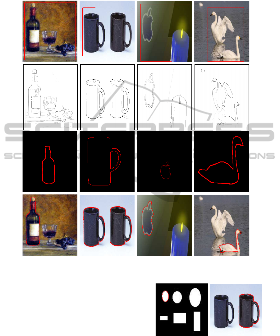
Figure 4: A sample of the results on the ETHZ dataset; row 1: initial curve; row 2: edge contours; row 3: shape model; row
4: final curve position.
shape priors generally require pose parameters esti-
mation and, hence, a close initialization is needed
which is often impractical. In Fig. 5, we show the
results obtained on two different test images using
the GAC model with a template matching shape prior
term as in (Paragios et al., 2002). For both images,
the template used actually corresponds to one of the
objects in the image, the smallest ellipse in the first
image and the black cup to the right of the second
image. Using one of the desired objects as the tem-
plate simplifies the problem for shape priors because
this forgoes the need to optimize with respect to the
pose parameters. As expected, the contours evolved
towards the objects correspondingto the templates but
missed all the other desired object instances.
(a) (b)
Figure 5: Results using the GAC model with a shape prior
term: (a,b) final curve positions.
Tracking Example: In this experiment, depicted in
Fig. 6, we investigate the tracking of both the left ven-
tricle cavity (first row) and the right ventricle (second
VISAPP 2012 - International Conference on Computer Vision Theory and Applications
246

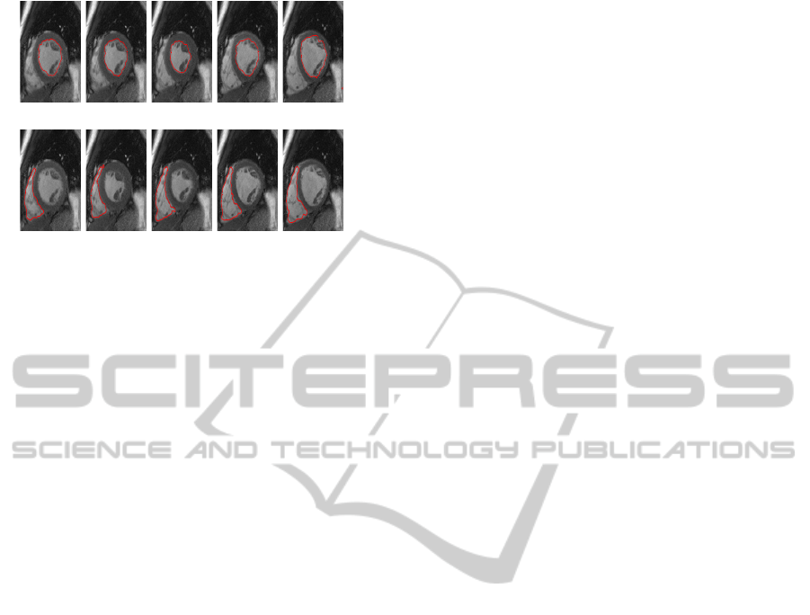
f5 f6 f11 f15 f25
f5 f10 f13 f17 f24
Figure 6: Tracking of both the left ventricle cavity (first
row) and the right ventricle (second row) in an MR se-
quence containing 25 frames (fx depicts frame x). For each
frame, the model distributions were learned from the result
of the previous frame. The first frame of the sequence was
segmented manually.
row) using the curvature as feature. For each frame,
the model distributions were learned from the result
of the previous frame. The first frame of the sequence
was segmented manually. Based on the learned out-
line pattern, the proposed method succeeds to distin-
guish between the left and the right ventricles in the
considered sequence.
5 CONCLUSIONS
We proposed an active contour edge-based functional
which measures the similarity between the curvature
distribution on the curve and a learned model dis-
tribution. The minimization of the ensuing Euler-
Lagrange equation, implemented via level sets, lead
to an evolution flow which is viewed as a geodesic
active contour with a variable stopping function. This
flow drives the active curve until it settles on the
boundaries of interest, i.e., boundaries on which the
curvature follows the model distribution. The formu-
lation is fundamentally different from region-based
schemes which cannot distinguish between regions
having the same image distributions. Several exper-
iments confirmed that the proposed method outper-
forms region and edge based formulations in adverse
conditions.
REFERENCES
Ben Ayed, I., Li, S., and Ross, I. (2009). A statistical over-
lap prior for variational image segmentation. Interna-
tional Journal of Computer Vision, 85(1):115–132.
Ben Ayed, I., Mitiche, A., and Belhadj, Z. (2005). Multire-
gion level set partitioning on synthetic aperture radar
images. IEEE Transactions on Pattern Analysis and
Machine Intelligence, 27(5):793–800.
Ben Ayed, I., Mitiche, A., and Belhadj, Z. (2006). Po-
larimetric image segmentation via maximum likeli-
hood approximation and efficient multiphase level
sets. IEEE Transactions on Pattern Analysis and Ma-
chine Intelligence, 28(9):1493–1500.
Ben Ayed, I., Mitiche, A., Salah, M. B., and Li, S. (2010).
Finding image distributions on active curves. In
CVPR, pages 3225–3232.
Berg, A., Berg, T., and Malik, J. (2005). Shape matching
and object recognition using low distortion correspon-
dance. In CVPR.
Boykov, Y. and Funka Lea, G. (2006). Graph cuts and effi-
cient N-D image segmentation. International Journal
of Computer Vision, 70(2):109–131.
Caselles, V., Kimmel, R., and Sapiro, G. (1997). Geodesic
active contours. International Journal of Computer
Vision, 22(1):61–79.
Chan, T. and Vese, L. (2001). Active contours with-
out edges. IEEE Transactions on Image Processing,
10(2):266–277.
Chan, T. and Zhu, W. (2005). Level set based shape prior
segmentation. In Computer Vision and Pattern Recog-
nition, volume 2, pages 1164–1170.
Cremers, D., Osher, S., and Soatto, S. (2006). Kernel den-
sity estimation and intrinsic alignment for shape pri-
ors in level set segmentation. International Journal of
Computer Vision, 69(3):335–351.
Cremers, D., Rousson, M., and Deriche, R. (2007). A re-
view of statistical approaches to level set segmenta-
tion: Integrating color, texture, motion and shape. In-
ternational Journal of Computer Vision, 72(2):195–
215.
Cremers, D., Sochen, N., and Schnorr, C. (2003). To-
wards recognition-based variational segmentation us-
ing shape priors and dynamic labeling. In Interna-
tional Conference on Scale Space Theories in Com-
puter Vision, volume 2695, pages 388–400.
Do Carmo, M. P. (1976). Differential geometry of curves
and surfaces. Prentice Hall.
Ferrari, V., Jurie, F., and Schmid, C. (2009). From images
to shape models for object detection. International
Journal of Computer Vision.
Ferrari, V., Tuytelaars, T., and Gool, L. V. (2006). Object
detection by contour segment networks. In European
Conference on Computer Vision (ECCV),.
Foulonneau, A., Charbonnier, P., and Heitz, F. (2006).
Affine-invariant geometric shape priors for region-
based active contours. IEEE Transactions on Pattern
Analysis and Machine Intelligence, 28(8):1352–1357.
Foulonneau, A., Charbonnier, P., and Heitz, F. (2009).
Multi-reference shape priors for active contours. In-
ternational Journal of Computer Vision, 81(1):68–81.
Freedman, D. and Zhang, T. (2004). Active contours for
tracking distributions. IEEE Transactions on Image
Processing, 13(4):518–526.
EXTRACTION OF REGION BOUNDARY PATTERNS WITH ACTIVE CONTOURS
247

Holtzman-Gazit, M., Kimmel, R., Peled, N., and Goldsher,
D. (2006). Segmentation of thin structures in volu-
metric medical images. IEEE Transacions on Image
Processing, 15(2):354–363.
Kass, M., Witkin, A. P., and Terzopoulos, D. (1988).
Snakes: Active contour models. International Jour-
nal of Computer Vision, 1(4):321–331.
Kichenassamy, S., Kumar, A., Olver, P. J., Tannenbaum, A.,
and Yezzi, A. J. (1995). Gradient flows and geometric
active contour models. In ICCV, pages 810–815.
Lecellier, F., Jehan-Besson, S., Fadili, J., Aubert, G., and
Revenu, M. (2009). Optimization of divergences
within the exponential family for image segmentation.
In SSVM, pages 137–149.
Leventon, M. E., Grimson, W. E., and Faugeras, O. (2000).
Statistical shape influence in geodesic active contours.
In Conference on Computer Vision and Pattern Recog-
nition, volume 1, pages 316–323.
Li, C., Xu, C., Gui, C., and Fox, M. D. (2005). Level set
evolution without re-initialization: A new variational
formulation. In Computer Vision and Pattern Recog-
nition.
Mansouri, A. and Mitiche, A. (2002). Region tracking via
local statistics and level set pdes. In IEEE Interna-
tional Conference on Image Processing, volume III,
pages 605–608, Rochester, NY, USA.
Mansouri, A., Mitiche, A., and Vazquez, C. (2006). Mul-
tiregion competition: A level set extension of region
competition to multiple region partioning. Computer
Vision and Image Understanding, 101(3):137–150.
Martin, D., Fowlkes, C., and Malik, J. (2004). Learn-
ing to detect natural image boundaries using local
brightness, color, and texture cues. IEEE Transac-
tions on Pattern Analysis and Machine Intelligence,
26(5):530–549.
Michailovich, O. V., Rathi, Y., and Tannenbaum, A. (2007).
Image segmentation using active contours driven by
the Bhattacharyya gradient flow. IEEE Transactions
on Image Processing, 16(11):2787–2801.
Mitiche, A. and Ayed, I. B. (2010). Variational and Level
Set Methods in Image Segmentation. Springer, 1st edi-
tion.
Mortensen, F. N. (2008). Progress in Autonomous Robot
Research. Nova Science Publishers.
Myronenko, A. and Song, X. B. (2009). Global ac-
tive contour-based image segmentation via probability
alignment. In CVPR, pages 2798–2804.
Paragios, N. and Deriche, R. (2002). Geodesic active re-
gions and level set methods for supervised texture seg-
mentation. International Journal of Computer Vision,
46(3):223–247.
Paragios, N., Mellina-Gottardo, O., and Ramesh, V. (2004).
Gradient vector flow fast geometric active contours.
IEEE Transactions on Pattern Analalysis and Ma-
chine Intelligence, 26(3):402–407.
Paragios, N., Rousson, M., and Ramesh, V. (2002). Match-
ing distance functions: A shape to area variational ap-
proach for global to local registration. In European
Conference in Computer Vision (ECCV), pages 775–
790.
Rousson, M. and Cremers, D. (2005). Efficient kernel den-
sity estimation of shape and intensity priors for level
set segmentation. In MICCAI, pages 757–764.
Salah, M. B., Mitiche, A., and Ayed, I. B. (2010). Effective
level set image segmentation with a kernel induced
data term. IEEE Transactions on Image Processing,
19(1):220–232.
Samson, C., Blanc-Feraud, L., Aubert, G., and Zerubia, J.
(2000). A level set model for image classification. In-
ternational Journal of Computer Vision, 40(3):187–
197.
Sethian, J. A. (1999). Level set Methods and Fast Marching
Methods. Cambridge University Press.
Vazquez, C., Mitiche, A., and Laganiere, R. (2006). Joint
segmentation and parametric estimation of image mo-
tion by curve evolution and level sets. IEEE Trans-
actions on Pattern Analysis and Machine Intelligence,
28(5):782–793.
Zhu, S. C. (2003). Statistical modeling and conceptualiza-
tion of visual patterns. IEEE Transactions on Pattern
Analysis and Machine Intelligence, 25(6):691–712.
Zhu, S. C. and Yuille, A. (1996). Region competition:
Unifying snakes, region growing, and Bayes/MDL
for multiband image segmentation. IEEE Transac-
tions on Pattern Analysis and Machine Intelligence,
118(9):884–900.
VISAPP 2012 - International Conference on Computer Vision Theory and Applications
248