PARAMETER AND CONFIGURATION ANALYSIS FOR

NON-LINEAR POSE ESTIMATION WITH POINTS AND LINES

Bernhard Reinert, Martin Schumann and Stefan Mueller

Institute of Computational Visualistics, University of Koblenz, Koblenz, Germany

Keywords:

Camera Pose Tracking, Model Features, Correspondences, Non-linear Optimization.

Abstract:

In markerless model-based tracking approaches image features as points or straight lines are used to estimate

the pose. We introduce an analysis of parametrizations of the pose data as well as of error measurements

between 2D image features and 3D model data. Further, we give a review of critical geometrical conﬁgurations

as they can appear on the input data. From these results the best parameter choice for a non-linear pose

estimator is proposed that is optimal by construction to handle a combined input of feature correspondences

and works on an arbitrary number and choice of feature type. It uses the knowledge of the 3D model to analyze

the input data for critical geometrical conﬁgurations.

1 INTRODUCTION

Model-based camera pose tracking is the process of

estimating the viewing position and orientation of a

camera by establishing 2D-3D correspondences be-

tween features of the model and the camera image.

Estimating the pose can be done by using linear or

non-linear solutions. Most pose algorithms origi-

nate from the domain of linear solutions and oper-

ate on point or line features. Combining both fea-

ture types has been done, but no complete comparison

of parametrization and error measurements for non-

linear solutions is available. Further, a priori model

knowledge should be used to improve stability of a

combined solution.

We provide a discussion on possible parametriza-

tions of the camera pose, including its constraints

which must be taken into account during or after the

optimization process as well as on several error mea-

surements for the feature correspondences to be min-

imized by the optimization process. Further, we give

a review of critical conﬁgurations as they are known

to cause ambiguous results on the input geometry of

points and lines. From these results we propose the

best parameter choice for a non-linear pose estima-

tor that is optimal by construction for the acceptance

of point and line correspondences in arbitrary com-

bination and number. The estimator takes account

of critical conﬁgurations of the input data by using

the knowledge of the 3D model and selecting the best

miminal correspondence set for a stable solution. We

investigate the behaviour on variable input types and

numbers of correspondences, as well as the inﬂuence

of noise on the robustness of the pose.

2 RELATED WORK

The problem of camera pose estimation with 2D-

3D correspondences of points is known as the

perspective-n-point problem (PnP) (Fischler and

Bolles, 1981). There are several approaches to the so-

lution of P3P surveyed and compared for their numer-

ical stability by (Haralick et al., 1994). While these

linear solutions work on a ﬁxed number of three point

correspondences, (Lepetit et al., 2009) introduce vir-

tual control points to make possible a solution for ar-

bitrary numbers of point correspondences (PnP) with

linear complexity. Another linear solution for any

number of point or line correspondences is given by

(Ansar and Daniilidis, 2003) but does not work on

both types of features simultaneously.

Most of the non-linear solutions are based

on classical iterative algorithms of optimization,

like the Gauss-Newton- or Levenberg-Marquardt-

Method. Non-linear pose with line correspondences

has been estimated by (Kumar and Hanson, 1994)

who analyzed the inﬂuence of certain line represen-

tations on the optimization process. A solution using

arbitrary line traits on an object is shown by (Lowe,

1991). Possible error measurements for point corre-

271

Schumann M., Reinert B. and Mueller S..

PARAMETER AND CONFIGURATION ANALYSIS FOR NON-LINEAR POSE ESTIMATION WITH POINTS AND LINES.

DOI: 10.5220/0003827402710276

In Proceedings of the International Conference on Computer Vision Theory and Applications (VISAPP-2012), pages 271-276

ISBN: 978-989-8565-04-4

 2012 SCITEPRESS (Science and Technology Publications, Lda.)

spondences were analyzed by (Lu et al., 2000), who

also proposed a new possibility requiring fewer itera-

tions. In (Dornaika and Garcia, 1999) points and lines

are combined under an extension of the well-known

POSIT algorithm with additional optimization.

Joint usage of point and line correspondences ex-

ists in the ﬁeld of linear solutions and to a lesser extent

in non-linear approches. But most authors analyze

one parametrization and a single error measurement

only, when solving for the camera pose. So in sec-

tions 4, 5 and 7 we will ﬁrst give a full analysis of

error measurements and parametrizations to ﬁnd the

best ﬁtted parameters for constructing combined non-

linear pose. An overview of critical conﬁgurations for

points is given by (Fischler and Bolles, 1981), where

(Wolfe et al., 1991) prove the number of solutions for

P3P geometrically as (Hu and Wu, 2002) and (Gao

and Tang, 2006) do for P4P. An example for critical

line conﬁgurations is given by (Christy and Horaud,

1999). We will address the problem of recognizing

such conﬁgurations in section 9.

3 DEFINITIONS

The pose problem can be described as the estima-

tion of the extrinsic camera parameters relative to a

known reference coordinate system, i.e. the world

coordinate system, from given correspondences be-

tween 2D features ~q of a camera image and 3D fea-

tures ~p of a synthetic model. The coordinate system

of a value is identiﬁed by a superscript w for world-, c

for camera-, i for image- and p for pixel-coordinate-

system. For all coordinate systems, the normalized

vector of ~p is denoted by

ˆp. The camera pose is rep-

resented in combination as a tuple consisting of a rota-

tion matrix R ∈ R

3x3

and a translation vector

t ∈ R

C :





and represents the transformation of a point

~p between world- and camera-coordinate-system as

= R

t. The intrinsic camera matrix K is as-

sumed to be known by calibration. Hence, given a

world point

and K, its pixel coordinates

can be

calculated by perspective projection. A point corre-

spondence between the world point

and the pixel

point

is represented by a tuple k





The line features in the camera images are deﬁned

as straight lines l : (φ

,ρ

) with inﬁnite extent. φ

represents the angle between the line normal and the

y-axis of the pixel coordinate system and ρ

is the

orthogonal distance of the line from the image origin.

Hence, for each point

∈ l it holds

cosφ

+ sinφ

= ρ

. (1)

A straight line correspondence is represented by two

world points

and

(typically start- and endpoint)

of the model line and an image line l

: (φ

,ρ

) by a

tuple k



(

),l



4 ERROR MEASUREMENTS FOR

POINTS

Since the aim is to minimize the distance between

the transformed model feature and camera image fea-

ture, error measurements, i.e. residuals, for corre-

spondences have to be deﬁned. We investigated three

different point residuals which measure the error in

different coordinate-systems (Figure 1).

The well-known Reprojection-Error measures

the distance between the image feature

and the

model feature

after its projection to the image

plane in pixel-coordinates. Hence, the residual for

each correspondence k

becomes

−



− q



. (2)

The Object-Space-Error measures the distance

in camera-coordinates and was introduced by (Lu

et al., 2000). To recover the depth for the image fea-

ture, its normalized sight vector

(i.e. the connect-

ing vector from the camera center to the feature) is

projected onto the sight vector of the model

. The

resulting scalar is used to scale the normalized sight

vector of the image

and both sight vectors are then

compared based on their camera coordinates. The

residual per correspondence k

becomes





−





. (3)

It has to be noted that points whose projections on the

image plane are the same produce greater residuals

for greater distances from the image plane, i.e. are

not depth invariant.

The Normal-Space-Error also measures the dis-

tance in the camera-coordinates. From the image fea-

ture

two orthogonal normals

and

can be cre-

ated, describing the direction of the sight vector of the

image in camera-coordinates. The dot product of the

normalized normals and the sight vector of the model

provides a measurement between image and model

features and the residual per correspondence k

be-

comes









. (4)

The Normal-Space-Error is not depth invariant as

well.

VISAPP 2012 - International Conference on Computer Vision Theory and Applications

272

Figure 1: Error measurements for points. Shown are the

camera coordinate system c, the image plane I, the vectors

for model and image feature

and

, the normals of the

Normal-Space-Error ~n

and ~n

together with their projec-

tion on

and the error measurements~r

,~r

and~r

AELE

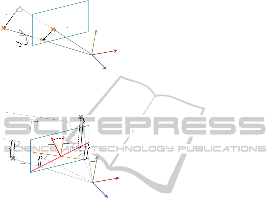
Figure 2: Error measurements for lines. Shown are the

camera coordinate system c, the image plane I, the model

and image feature

and l

, the line ℓ

, their normals

and

ℓ

, the plane E

with its normal

and the components

of the error measurements~r

,~r

and~r

5 ERROR MEASUREMENTS FOR

LINES

We investigated three different line residuals which

measure the error in different coordinate-systems

(Figure 2).

The Angle-/Distance-Error measures the differ-

ences of the angles and the distances of the image and

model feature. The start- and endpoint of the model

feature are transformed into their pixel points

to compute the conjunctive line ℓ : (ϕ

), which is

compared to the image line l

. The residual per cor-

respondence k

therefore becomes



− φ

− ρ



. (5)

Noteable for this error measurement is that the dimen-

sions of the angle and the distance are not equal.

The Line-Error measures the distances of the

projected start- and endpoint

to the image line

and is used, among others, by Lowe (Lowe, 1991).

Hence, from Eq. 1 the residual for each correspon-

dence k

becomes



cosφ

+ sinφ

− ρ

cosφ

+ sinφ

− ρ



. (6)

The Plane-Error can be regarded as the Object-

Space-Error extension for straight lines, i.e. the depth

recovery of the image feature, and is used e.g. by

(Kumar and Hanson, 1994). The optical center and

the image line in camera coordinates l

deﬁne a plane

with normal



cosφ

sinφ

−ρ



. For

start- and endpoint in camera coordinates

the

distance to this plane can be computed. The residual

for each correspondence k

becomes:









. (7)

Similar to the Object-Space-Error, the Plane-Error is

not depth invariant.

6 OPTIMIZATION

The residuals of all correspondences are joined in one

combined residual~r. The pose parameters for transla-

tion

and rotation

are combined in the parameter

vector~a. The objective is to minimize the sum of the

squared entries of this combined residual in terms of

the pose parameters~a.

argmin

∑

j=0

(8)

To solve this problem standard optimization tech-

niques are used so that the parameter vector is turned

into a sequence h~a

i. Since the Gauss-Newton op-

timization is comparatively fast but does not guar-

antee convergence and Gradient-Descent optimiza-

tion is slow but guarantees convergence, we used the

Levenberg-Marquardt optimization that is commonly

known as a technique which guarantees convergence

but is still comparatively fast. The iteration rule is

i+1

= ~a

δ with

δ =



(~a

)

(~a

) + λD



−1

(~a

)~r(~a

), (9)

D = diag



(~a

)

(~a

)



and J

the Jacobian matrix

of~r. We found the initial value of λ = 10

−3

and an

alteration rule of λ

= λ

i−1

/10 for a residual decrease

and λ

= λ

i−1

∗ 10

with w ∈ N for a residual increase

of the last step to work best.

PARAMETER AND CONFIGURATION ANALYSIS FOR NON-LINEAR POSE ESTIMATION WITH POINTS AND

LINES

273

7 PARAMETRIZATION

We also investigated the inﬂuence and conditions

of different parametrizations of the pose. Different

parametrizations of the translation vector

do not

hold any major differences and it is therefore repre-

sented by three scalars t

, t

and t

, describing the

translation in camera coordinates; the translation pa-

rameter vector is

For rotation parametrization we investigated four

different alternatives. All rotations are described by

their corresponding transformation matrices R and

have to fulﬁll certain rotation properties since R ∈

SO(R, 3), i.e. the special orthogonal group proper-

ties (SOP). In general, these properties can be assured

at various stages of the optimization process:

I. prior to optimization

By choosing an appropriate rotation parametriza-

tion the SOP can be assured partly or completely

prior to the optimization process.

II. during optimzation

By adding the SOP as additional elements to the

residual vector, these properties are optimized

with the other residuals. A drawback of this al-

ternative is that with the presence of imperfect or

false correspondences the properties are not en-

forced but only minimized according to the least

squares approach of the optimization.

III. after optimization

By employing the singular value decomposition,

a rotation matrix

R can be computed from the es-

timated transformation matrix R that assures the

SOP and is similar to R.

These three possibilities are not exclusionary; alter-

native II. has to be combined with alternative III. for

the SOP to be fulﬁlled.

The parameter vector of the

Matrix-Parametrization is





. The

transformation matrix is composed of three vectors

k ∈ R













(10)

Advantageous is that the transformation matrix and its

derivatives can efﬁciently be computed. However, the

SOP are not enforced and alternatives II. and III. have

to be employed: Matrix R should form an orthonor-

mal basis and have determinant +1. Both constraints

are added to the residual.

The parameter vector of the Euler-Angles-

Parametrization is





. The ro-

tation matrix is composed of three consecutive rota-

tions around the coordinate axis:

= R







− s

−c

+ c

−c







(11)

with c

= cosφ

, c

= cosφ

, c

= cosφ

, s

= sinφ

and s

= sinφ

. The SOP are therefore en-

forced prior to optimization. Disadvantageous is the

well-known gimbal lock and the extensive usage of

trigonometric functions.

The parameter vector of the Quaternion-

Parametrization is



w x y z



. The

transformation matrix is composed by using a unit

quaternion q : (w,x,y,z) ∈ H with rotation axis

v = (x,y,z)

and rotation angle φ = 2arccosw:





+ x

− y

− z

2(xy− wz) 2(xz+ wy)

2(xy+ wz) w

− x

+ y

− z

2(yz− wx)

2(xz− wy) 2(yz+wx) w

− x

− y

+ z





(12)

Since q has to be a unit quaternion, the SOP are not

completely enforced and alternatives II. and III. have

to be employed with |q| = 1 added to the residual. It is

cogitable to substitute e.g. w in terms of x, y and z as

w =

1− x

− y

− z

. Disadvantageous with quater-

nions is that there exist complex solutions for w.

The parameter vector of the Rodrigues’-

Formula-Parametrization is



x y z



The rotation matrix is composed by a rotation axis

~v = (x,y, z)

and a rotation angle φ = |~v|:







cosφ + x

xyc

− zs

− xzc

+ xyc

cosφ + y

yzc

− xs

xzc

− ys

+ yzc

cosφ + z







(13)

with c

1−cosφ

, s

sinφ

and φ =

+ y

+ z

or in case of φ = 0 it holds R

= I

. The SOP are

guaranteed by this parametrization.

8 SCALING

In general, due to discretization and erroneous match-

ing we cannot rely on perfect correspondences.

Therefore, the weight of each correspondence be-

comes crucial for the estimated result as unequal

weights shift the minima of the squared sum (Eq. 8)

to different positions. In order to ﬁnd the optimal

least-squares value for all given correspondences, the

dimensions of all entries of the residual have to be

equal. Except for the Angle-/Distance-Error, all er-

ror measurements and SOP have a dimension of ei-

ther pixel or camera points, and scaling factors for the

corresponding other dimension can easily be derived

using the given camera matrix.

VISAPP 2012 - International Conference on Computer Vision Theory and Applications

274

9 GEOMETRICAL

CONFIGURATION

The pose problem can be solved with a ﬁnite number

of solutions when at least three point correspondences

are known (Fischler and Bolles, 1981), but there may

exist up to four possible solutions. Using four cor-

respondences the pose can be solved with a unique

solution only when the correspondences are in copla-

nar conﬁguration (Gao and Tang, 2006). Otherwise

up to ﬁve solutions are possible. For ﬁve correspon-

dences still up to two solutions may occur when they

are not in coplanar conﬁguration. Thus, when using

a minimal number of four or ﬁve correspondences a

coplanar conﬁguration should be assured to prevent

multiple solutions. Additionally, the correspondences

should not be in degenerate conﬁguration, i.e. they

are linearly dependent. For six or more linearly in-

dependent point correspondences in arbitrary conﬁg-

uration the pose problem becomes unambiguous. For

coplanar lines a ﬁnite solution is also feasible with at

least three lines. For a non-coplanar conﬁguration at

least four lines are required. They must not be in de-

generate conﬁguration, i.e. more than two lines are

parallel or intersect in one point (Christy and Horaud,

1999). Due to the known 3D data of the model, for

each correspondence the geometrical relationship to

the others in the correspondence set can be surveyed.

Table 1: Possible number of solutions for several numbers

of point correspondences and their conﬁguration.

#correspondences non-coplanar coplanar

3 - 4

4 5 1

5 2 1

≥6 1 1

To check for linear dependency, i.e. three points

located on one straight line, the dot product of the

normalized direction vectors from one point to the

other two is calculated. If it becomes close to 1, the

correspondence will be rejected for pose estimation.

To check for coplanarity, a plane is calcuated from

the normalized direction vectors of three points. The

vector of the remaining fourth point is then inserted

into the equation of the plane. If the four points are

in coplanar conﬁguration, the solution will be unique

and the correspondences are accepted as input data.

For straight lines linearly dependent conﬁgura-

tions occur if more than two lines are parallel or inter-

sect in one point. Parallelism is checked for by cal-

culating the dot product of the normalized direction

vectors of the lines. If all products are close to 1, the

lines are linearly dependent and the line correspon-

dences will be rejected. To check for a common inter-

section point, the intersection point of each line pair

is calculated respectively. If two or more intersection

points exist and the euclidean distance between these

points is below a predeﬁned threshold, the lines are

collinear and will not be candidates for input data.

10 RESULTS

We tested combinations of error measurements and

parametrizations using points, lines and mixed corre-

spondences for the non-linear estimator. For the ex-

periments with synthetical data at an image resolution

of 640 x 480 pixel we used a unit cube around the ori-

gin; the initial camera pose was (0, 0,−5)

. In the

test sequence the camera was rotated by 30

◦

about the

axes of the world coordinate system and translated by

the vector (1, 1,1)

. Using this pose the correspon-

dences were established by perspective projection of

the 3D model features to the image plane, followed

by adding uniformly distributed noise in the range of

[0,10] pixel of displacement in arbitrary direction. We

regarded mean error and standard deviation between

real and estimated pose for translation, rotation and

number of iterations over 100.000 tests.

On points the comparison of error measurements

indicates that the image based Reprojection-Errorper-

forms more accurately than the Object-Space-Error

and Normal-Error for all possible combinations with

pose parametrizations. This can be explained by a

potentionally higher weighting of points in the ob-

ject space when they are more distant from the cam-

era center. The number of iterations is compara-

ble for all types of error measurement. Concerning

parametrization, Euler computation is slightly slower

while quaternions perform somewhat better, but lead

to less accurate translation estimation. For line cor-

respondences, the Angle-Distance-Error causes bad

pose results and a higher computation time. Line- and

Plane-Error are comparable for all parametrizations,

regarding accuracy and speed. Quaternions show a

slightly better computational performance.

Therefore, we propose Rodrigues’-Formular-

Parametrization together with Reprojection- and

Line-Error for combined non-linear pose estimation.

This combination shows the smallest pose error with-

out noticeable decrease in speed. In addition, using

pixel space error for both feature types, scaling is

not necessary to compensate for depth differences be-

tween the correspondences. The Rodrigues’-Formula

proves to be the best parametrization because inde-

pendent of the chosen error measurement it does not

inﬂuence pose accuracy. It is gimbal-lock free and

PARAMETER AND CONFIGURATION ANALYSIS FOR NON-LINEAR POSE ESTIMATION WITH POINTS AND

LINES

275

complies with the constraints of a rotation matrix by

deﬁnition. Thus, there is no need for additional en-

tries in the residual vector to be minimized during op-

timization and no singular value decomposition has to

be run afterwards to correct the result.

We also tested the inﬂuence of combining both

feature types under our proposed parameters. We

combined a minimal number of six correspondences

of one feature type with several numbers of the other

one and added several levels of noise. A pose esti-

mated by points is improved in rotation and transla-

tion by adding line correspondences independently of

the displacement error in the given point correspon-

dences. The improvement of the estimate converges

when at least six line correspondences are added to

the point correspondences. In the opposing case ad-

ditional point correspondences show a positive im-

pact on the exactness of a pose estimated with lines

only when the underlying line correspondences are

very noisy. This is due to a generally higher stability

of line features concerning displacement error. Point

features will be affected more strongly by growing

correspondence errors than lines. We can state that

a combination of point and line features is useful in

practical application to stabilize the estimated pose,

especially when there is only a minimal set of corre-

spondences available.

The resulting optimal estimator was successfully

run on a real test scene for veriﬁcation of real-time

capabilities. The estimator pass for combined input

with point and line correspondences took about 1 ms

CPU time. The combination of both feature types did

not reduce computational speed, thus real time appli-

cation is ensured. Further, it could be seen that the

required number of iterations depends to a large de-

gree on the error level of the correspondences, while

it is hardly inﬂuenced by the total number of corre-

spondences.

11 CONCLUSIONS

We analyzed the best parameter choice for a non-

linear pose estimator when using a combined input

of point and line correspondences. Test results show

that the error measurement in pixel coordinates is su-

perior to the error in object space for points as well

as for lines. Further, it is proved that a parametriza-

tion may be chosen which fulﬁlls the constraints of a

rotation matrix without requiring additional computa-

tional load. For points and lines this is the case with

Rodrigues parametrization. An optimal non-linear

estimator can be constructed by these propositions

working on an arbitrary number and choice of feature

type with a minimal set of three correspondences. The

estimator will improve the pose by considering the

conﬁguration of the combined input data and select-

ing those point and line correspondences only, which

are proved to deliver unambiguous results.

ACKNOWLEDGEMENTS

This work was supported by grant no. MU 2783/3-1

of the German Research Foundation (DFG).

REFERENCES

Ansar, A. and Daniilidis, K. (2003). Linear Pose Estimation

from Points or Lines. In IEEE Transactions on Pattern

Analysis and Machine Intelligence, volume 25, pages

578–589.

Christy, S. and Horaud, R. (1999). Iterative Pose Compu-

tation from Line Correspondences. Computer Vision

and Image Understanding, 73:137–144.

Dornaika, F. and Garcia, C. (1999). Pose Estimation using

Point and Line Correspondences. Real-Time Imaging,

5:215–230.

Fischler, M. A. and Bolles, R. C. (1981). Random sample

consensus: a paradigm for model ﬁtting with appli-

cations to image analysis and automated cartography.

Communications of the ACM, 24:381–395.

Gao, X.-S. and Tang, J. (2006). On the Probability of the

Number of Solutions for the P4P Problem. ournal of

Mathematical Imaging and Vision, 25:79–86.

Haralick, B., Lee, C.-N., Ottenberg, K., and Nlle, M.

(1994). Review and analysis of solutions of the three

point perspective pose estimation problem. Interna-

tional Journal of Computer Vision, 13(3):331–356.

Hu, Z. Y. and Wu, F. C. (2002). A Note on the Number

of Solutions of the Noncoplanar P4P Problem. IEEE

Transactions on Pattern Analysis and Machine Intel-

ligence, 24:550–555.

Kumar, R. and Hanson, A. (1994). Robust methods for es-

timating pose and a sensitivity analysis. Computer Vi-

sion Graphics and Image Processing: Image Under-

standing, 60(3):313–342.

Lepetit, V., Moreno-Noguer, F., and Fua, P. (2009). EPnP:

An Accurate O(n) Solution to the PnP Problem. Inter-

national Journal Of Computer Vision, 81:155–166.

Lowe, D. (1991). Fitting parameterized three-dimensional

models to images. In IEEE Transactions on Pattern

Analysis and Machine Intelligence, volume 13(5),

pages 441–450.

Lu, C.-P., Hager, G., and Mjolsness, E. (2000). Fast and

Globally Convergent Pose Estimation from Video Im-

ages. IEEE Transactions on Pattern Analysis and Ma-

chine Intelligence, 22(6):610–622.

Wolfe, W. J., Mathis, D., Sklair, C. W., and Magee, M.

(1991). The Perspective View of Three Points. IEEE

Transactions on Pattern Analysis and Machine Intel-

ligence, 13:66–73.

VISAPP 2012 - International Conference on Computer Vision Theory and Applications

276