LOW-RANK RADIOSITY USING SPARSE MATRICES
Eduardo Fern´andez
1
, Pablo Ezzatti
1
, Sergio Nesmachnow
1
and Gonzalo Besuievsky
2
1
Centro de C´alculo, Universidad de la Rep´ublica, Montevideo, Uruguay
2
Geometry and Graphics Group, Universitat de Girona, Girona, Spain
Keywords:
Radiosity, Real-time Global Illumination.
Abstract:
Radiosity methods are part of the global illumination techniques, which deal with the problem of generating
photorealistic images in 3D scenes with Lambertian surfaces. Low-rank radiosity is a O(nk) method, where
n is the number of polygons and k is the rank of the matrix used as a direct transport operator. This method
allows calculating, in real-time and with infinite bounces, the illumination of a scene with static geometry
and dynamic lighting. In this paper we present a new methodology for low-rank radiosity calculation based
on the use of sparse matrices, which significantly reduces the memory storage required and achieves speedup
improvements over the original low-rank method. Experimental analysis was performed in both traditional
computers and new graphics processing unit architectures.
1 INTRODUCTION
The radiosity method is a pioneering technique for
global illumination on scenes with Lambertian sur-
faces, which has been applied in many areas of design
and computer animation (Dutre et al., 2006).
Since the classic formulation of the radiosity tech-
nique in the decade of 1980, several iterative res-
olution methods have been proposed (Cohen et al.,
1993). These methods are not feasible for computing
realistic images in real-time (many bounces at 20 fps),
due to their iterative nature. After that, several other
methods have been proposed to achieve the real-time
computation of the global illumination, such as in-
stant radiosity (Keller, 1997), precomputed radiance
transfer (Sloan et al., 2002), radiance transport (Kon-
tkanen et al., 2006; Lehtinen et al., 2008) and photon
mapping (Wang et al., 2009), which have shown some
success using global illumination approximations.
By exploiting spatial coherence, the low-rank ra-
diosity method (LRR) (Fern´andez, 2009) allows
solving the real-time radiosity problem with infinite
bounces, for scenes with static geometry and dynamic
lighting, using a low memory storage approach. The
original LRR implementation used full matrices, and
the promising idea of generating sparse matrices was
previously pointed out, but it was not developed.
This work presents a new approach for the utiliza-
tion of sparse matrices in the LRR method. Specific
implementations of algorithms to solve the radiosity
problem in both traditional computer architectures
(CPU) and modern graphic processing units (GPU)
are introduced. The experimental results show that
the GPU implementation of the LRR method based on
sparse matrices has an acceleration factor greater than
four, compared with the full matrix approach of the
LRR method. These promising results demonstrate
that our approach is an alternative for real-time radio-
sity applications. Comparing to other strategies, LRR
ensures always a full global illumination solution be-
ing capable of dealing efficiently with environments
with significant indirect illumination contribution.
The rest of the article is organized as follows. Sec-
tion 2 introduces the radiosity problem and the pre-
vious work. The low-rank radiosity method is de-
scribed in Section 3. Section 4 introduces the utiliza-
tion of sparse matrices in LRR, and describes the im-
plementations of the proposed algorithms for sparse
low-rank radiosity in CPU and GPU. The experimen-
tal analysis is reported in Section 5. Finally, Section 6
summarizes the conclusions of the research and for-
mulates the main lines for future work.
2 THE RADIOSITY PROBLEM
This section starts by introducing the radiosity pro-
blem formulation. After that, the main proposals
found in the literature related with the pre-computed
radiosity and radiance transfer problem are reviewed.
260
Fernández E., Ezzatti P., Nesmachnow S. and Besuievsky G..
LOW-RANK RADIOSITY USING SPARSE MATRICES.
DOI: 10.5220/0003829402600267
In Proceedings of the International Conference on Computer Graphics Theory and Applications (GRAPP-2012), pages 260-267
ISBN: 978-989-8565-02-0
Copyright
c
 2012 SCITEPRESS (Science and Technology Publications, Lda.)

2.1 Problem Formulation
The radiosity problem is modeled by a Fredholm in-
tegral equation, the radiosity equation (1). In Equa-
tion 1, B(x) is the radiosity in the point x, E(x) is the
light emission in x, ρ(x) is the Lambertian diffuse re-
flectivity of x, and G(x, x
′
) is a geometric factor that
determines how much the radiosity in x
′
contributes
to the radiosity of x (Cohen et al., 1993).
B(x) = E(x) + ρ(x)
Z
S
B(x
′
)G(x,x
′
)dA
′
(1)
Any Fredholm equation can be transformed into a dis-
crete equation, which implies solving a linear system.
In the radiosity problem the linear system is expressed
by Equation 2, where I is the identity matrix with di-
mension n×n (n is the number of polygons), R is a
diagonal matrix that stores the reflectivity of the poly-
gons, F is the matrix with the form factors F
ij
–which
indicate the fraction of light reflected by the polygon
i that arrives to the polygon j–, B is a vector with the
radiosity value of each patch, and E is the vector with
the emission of each patch.
(I− RF)B = E (2)
This discrete equation can be also formulated through
the use of a direct transport operator T, which ex-
presses the direct transmission of light between two
surfaces of the scene. Using T, the discrete radiosity
equation (Equation 2) is expressed as (I− T)B = E.
Moreover, the operator G = (I − T)
−1
, is a global
transport operator relating the emitted light with the
final radiosity of the scene, B = GE. For scenes where
the geometry is fixed and only the light output varies,
the operators T and G are constant.
2.2 Related Work
The main class of elements used in light transport
includes the polygons, the parametric surfaces (Co-
hen et al., 1993), and the discrete points (Fasshauer,
2006). In all these cases it is possible to build oper-
ators T and G that indicate the transport relationship
between any pair of elements.
The O(n
2
) memory required to store T has been
clearly posed as a problem in early radiosity papers
(Cohen et al., 1988). Many solutions have been pro-
posed, such as two-level hierarchy (Cohen et al.,
1986), hierarchicalstructures (Hanrahan et al., 1991),
and wavelets (Gortler et al., 1993). The memory sav-
ings are determined by the spatial coherence of the
scenes, where it is highly probable that neighboring
elements i, j have similar transport values with many
other elements k of the scene, that is, T
ik
≈ T
jk
. In this
case, these values are considered equal, then, many
transport values can be replaced by a single value.
This is the main idea behind the hierarchical approx-
imation H(T) of any T operator, where H(T) is usu-
ally stored in O(n) memory. The balance between
the error introduced by the method and the memory
saved is highly convenient for most scenes. In these
works the calculation of B is done by iterative me-
thods, avoiding the need of computing H(G).
Recently, other kinds of methods that include
BRDF surfaces and the calculation of H(G) have
been developed. In (Kontkanen et al., 2006), the
BRDF operator (T) is transformed into H(T) through
the use of wavelets, and H(G) is calculated using the
Neumann series H(G) = I+ H(T) + H(T)
2
+ . .., by
removing all values of H(T)
n
smaller than a certain
threshold. After calculating the global incident radi-
ance of a scene, the BRDF function is applied again to
find an image from a particular point of view. Later, in
(Lehtinen et al., 2008) a meshless hierarchical repre-
sentation of the objects in the scene, built upon a hier-
archy of points, is performed. Each point consists of
a pair (position, normal) and has a radius of influence
related with the hierarchy level to which it belongs.
Using a hierarchical function basis, a sparse matrix
H(T) is generated by elimination of all terms below
a threshold, and a final sparse operator H(G − I) is
created, using also Neumann series.
Other methods to achieve real-time global illu-
mination are based on instant radiosity techniques
(Keller, 1997) and its variants (Laine et al., 2007),
but these methods compute only a few bounces.
In contrast, the LRR method proposed in this work
allows to solve the radiosity problem with infinite
bouncesand relatively small computational resources.
This result is based on the premise that when T is a
low-rank matrix, the operator G can be easily calcu-
lated, as it is explained in the next section.
3 THE LOW-RANK RADIOSITY
METHOD
It is very likely that the (RF) matrix included in Equa-
tion 2 has a low numeric rank. This is because each
row (RF)
i
is computed based on the scene view from
the element i, and most pairs of close patches have a
very similar view of the scene (Figure 1). Then (RF)
has many similar rows, which results in a reduction of
the numerical rank.
The rank reduction of (RF) matrices allows
approximating them by the product of two matrices
U
k
V
T
k
, both with dimension n×k (n≫k), without los-
ing relevant information about the scene.
LOW-RANK RADIOSITY USING SPARSE MATRICES
261

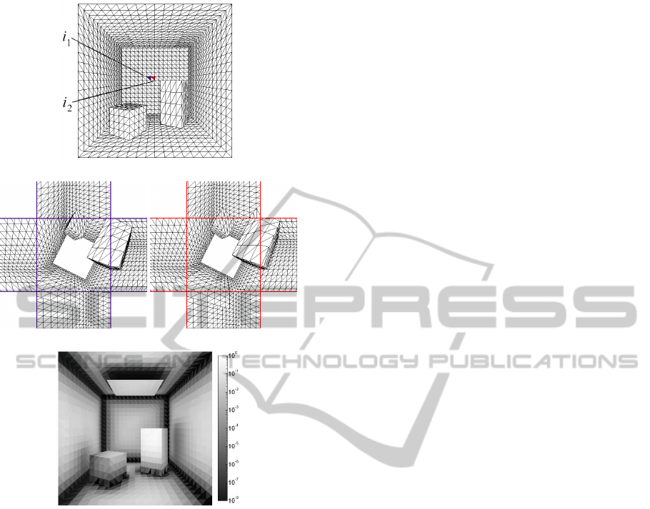
(a) Two close patches i
1
and i
2
.
(b) Hemicube view from i
1
. (c) Hemicube view from i
2
.
(d) Spatial coherence in the scene.
Figure 1: Close patches have similar views of the scene and
generate similar rows in (RF). In (d) the spatial coherence
of each patch is measured (darker means lower coherence).
3.1 Low-rank Approximation
The product U
k
V
T
k
generates a matrix with dimension
n×n and rank k. The memory space needed to store
U
k
and V
T
k
is O(nk), significantly less than the O(n
2
)
required to store the matrix (RF), especially when
n≫k. This memory saving allows reducing the space
needed to store the information for large scenes.
In the LRR equation (3), (RF) is replaced by the
low-rank approximation U
k
V
T
k
. The unknown is not
longer B, but an approximation
e
B of the radiosity.

I− U
k
V
T
k

e
B = E (3)
The matrix

I− U
k
V
T
k

is easily invertible using the
Sherman-Morrison-Woodbury formula (Golub and
Loan, 1996). Equation 4 shows the expression for
e
B.
e
B = E + U
k


I
k
− V
T
k
U
k

−1

V
T
k
E


(4)
In order to find
e
B through Equation 4, O(nk
2
) opera-
tions are required and O(nk) memory is needed.
In scenes with static geometry and dynamic light-
ing (i.e., only the independent term E varies in Equa-
tions 2 to 4), part of the computation can be executed
before the real-time stage. Equation 4 is transformed
into 5, where the n×k matrices Y
k
, U
k
, and V
k
are cal-
culated once. Thus, the real-time stage only has com-
plexity O(nk). This is an auspicious result in order to
develop a new methodology for real-time radiosity.
e
B = E − Y
k

V
T
k
E

, (5)
Y
k
= −U
k

I
k
− V
T
k
U
k

−1
Equation 5 can also be formulated as
e
B = GE, so
G = I − Y
k
V
T
k
is considered as the global operator
that manages the infinite bounces of light in a single
operation. This global operator is computed without
the use of Neumann series, as in (Kontkanen et al.,
2006; Lehtinen et al., 2008), taking advantage of the
fact that (RF) is a low-rank matrix.
3.2 U
k
and V
k
Calculation
U
k
and V
k
can be computed using factorization tech-
niques, such as singular value decomposition (SVD
or PCA) (Golub and Loan, 1996), CUR factoriza-
tion (Goreinov et al., 1997), and discrete transfor-
mations based on Fourier and wavelets (Press et al.,
2007). SVD is the only method that produces good
approximations to (RF) for low values of k, but it has
an O(n
3
) complexity. The other methods mentioned
have lower complexity orders, but they also produce
larger errors in the (RF) approximation.
To overcome the weakness of the traditional fac-
torization techniques, the Low-Rank Radiosity (LRR)
method proposed in (Fern´andez, 2009) uses the con-
cept of spatial coherence (Sutherland et al., 1974).
This method generalizes the two-level hierarchy me-
thodology (Cohen et al., 1986), where two meshes
with different granularity levels are generated for the
scene (a coarse mesh with k patches and a fine mesh
with n elements). Using these two meshes it is possi-
ble to build the n×k matrices U
k
and V
k
.
Both, the coarse and the fine meshes, can be uni-
form or nonuniform. In this paper, we proposed a
nonuniform coarse mesh that is adapted to the spatial
coherence of the scene. In the resulting algorithm,
named 2 Meshes with Spatial Coherence (2MSC), the
fine mesh is given, assuming that inside each element
there is spatial coherence, but the coarse mesh is built
taking care of the spatial coherence inside each patch.
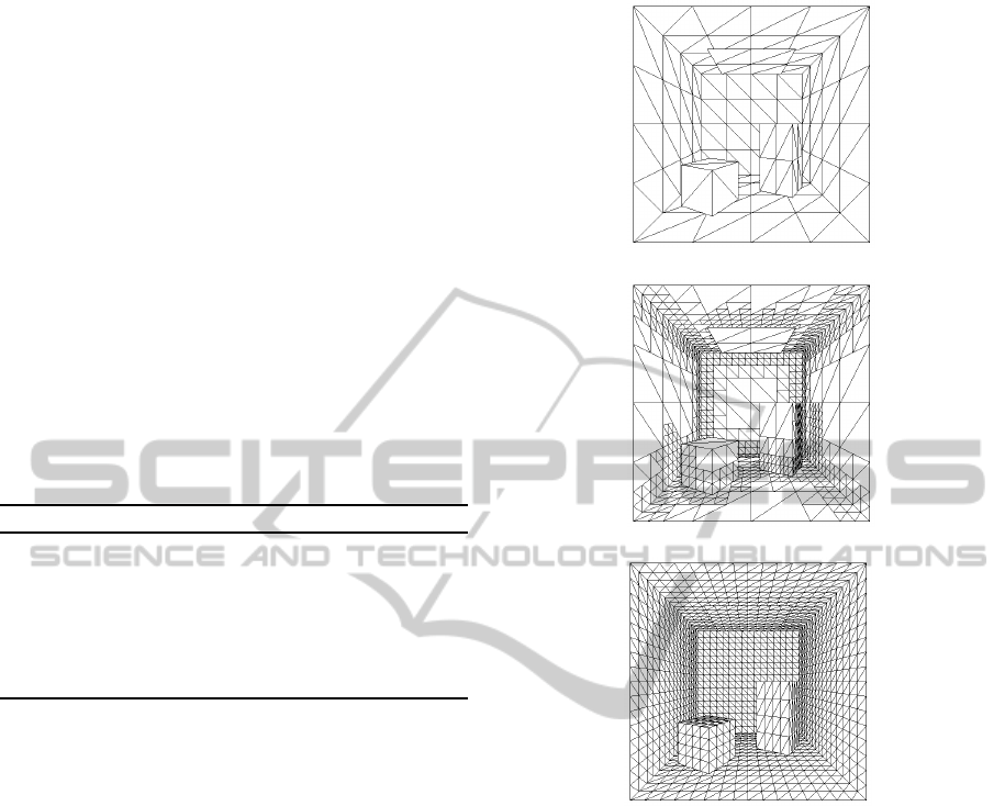
The 2MSC produces a nonuniform mesh, with
smaller patches in those areas with low spatial cohe-
rence. Algorithm 1 shows a top-down procedure for
GRAPP 2012 - International Conference on Computer Graphics Theory and Applications
262

creating the coarse mesh from a few large patches,
using the 2MSC algorithm. An initial set of large
patches are inserted into a list L (see Figure 2 (a)). Ev-
ery patch is taken from L, one at a time. All patches
without spatial coherence (i.e., when the inner scene
views vary more than a specified threshold) are split
into several subpatches, which are inserted into L.
The algorithm stops when the list L is empty (i.e.,
when all patches have spatial coherence), or when all
those patches without spatial coherence are smaller
than a predefined value (A
min
). The number of patches
(k) depends on the value of the parameter A
min
and
also depends on the procedure used to evaluate the
spatial coherence. Figure 2 (b, c) shows a coarse mesh
generated using the 2MSC algorithm and a fine mesh.
The discretization of the coarse mesh shown in Fig-
ure 2 (b) agree with the colors of spatial coherence
shown in Figure 1 (d), i.e., the darker the color, the
more need to split the surface.
Algorithm 1: 2MSC algorithm.
1: Store patches p in a list L.
2: while (L6={}) do
3: Remove a patch p from L.
5: if ¬(spatial coherence inside p) ∧ (Area(p) > A
min
)
6: Divide p in subpatches and store them in L.
7: end.
8: end.
After the scene meshes are defined, the matrices
U
k
and V
k
are built using the information from an as-
signment function P : e → p that gives, for each ele-
ment e in the fine mesh, the corresponding patch p in
the coarse mesh. The assignment can be defined by
inclusion (element e belongs to single patch p) or by
proximity (p is the closest patch to element e).
If P is defined by inclusion and all elements be-
longing to any patch have equal area, the construction
of matrices U
k
and V
k
follows Equation 6. There, F
ep
is the form factor between an element e of the scene
and the elements assigned to the patch p, and c
p
is the
number of elements assigned to p.
U
k
(e, p) = F
ep
/c
p
V
k
(e,P(e)) = 1 , V
k
(e, p) = 0 ∀p 6= P(e) (6)
Other methodologies can be applied to build the
matrices U
k
and V
k
. Besides using SVD factoriza-
tion, where the columns of both matrices are orthog-
onal, the columns of the matrix U
k
generated using
Equation 6 can also be orthogonalized using QR fac-
torization. After the QR factorization is performed,
a new matrix U
QR
is generated and V
k
can be re-
placed by V
QR
= (RF)
T
U
QR
. These methodologies
have been implemented by the authors to generate U
k
and V
k
, and the experiments showed no conclusive
(a) Original coarse mesh.
(b) Coarse mesh after 2MSC.
(c) Fine mesh.
Figure 2: Meshes used to compute U
k
and V
k
.
results about which is best method. In this paper, the
Equations in 6 were employed to build the matrices,
due to both the simplicity of building a low rank ap-
proximation of the (RF) matrices and the possibility
to build a sparse version of the V
k
matrix, as it is ex-
plained in the next section.
4 SPARSE MATRICES IN LRR
The 2MSC algorithm and the Equations 6 gene-
rate sparse matrices V
k
with dimension n×k, with
a unique non-zero entry in each row (corresponding
with the P(e) column). This section introduces an
O(k) storage methodology for the V
k
matrix, and an
implementation of the LRR method for both CPU and
GPU platforms.
LOW-RANK RADIOSITY USING SPARSE MATRICES
263

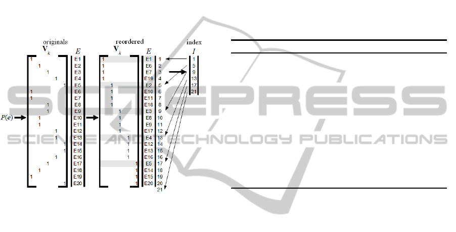
4.1 Compressing the Information in V
k
The rows of V
k
can be reordered, grouping them by
the column where the non-zero value is in (k dis-
joint groups are created, see Figure 3). Using ideas
from the compressed storage of sparse matrices (Bar-
rett et al., 1994), an index vector I can be defined. I
indicates that the rows of V
k
with a one in the first co-
lumn are placed from I
1
= 1 to I
2
−1, that the rows of
V
k
with a one in the second column are placed from I
2
to I
3
−1, and so on. The O(k) entries of I are enough
to define the matrix V
k
.
Figure 3: Construction of V
k
and I from the function P.
Once the vector I is built and the values in the vec-
tor E are reordered accordingly to the rows of V
k
, the
product V
T
k
E can be formulated as the sum in Equa-
tion 7. The i-th value of the vector V
T
k
E is the sum of
the values of E between the positions I
i
and I
i+1
− 1.

V
T
k
E

i
=
I
i+1
−1
∑
s=I
i
E
s
, ∀i,1 ≤ i ≤ k (7)
The previously presented results allow to conclude
that if V
k
is a sparse matrix with the stated proper-
ties, the matrix-vector product V
T
k
E can be computed
in O(n) operations (instead of the O(nk) operations
needed when V
k
is a full matrix).
4.2 Sparse LRR Implementation
In order to validate the theoretical results presented in
the previous subsection, two implementations of the
sparse LRR method were developed to solve the ra-
diosity problem with a sparse V
k
matrix generated by
Equations 6. Each implementation uses a different
hardware to perform the calculations: one uses a tra-
ditional CPU, and the other uses a GPU.
The LRR implementation in CPU uses the BLAS
library (Lawson et al., 1979), and Equation 7 is solved
sequentially. On the other side, the LRR implemen-
tation in GPU uses the CUBLAS implementation of
BLAS for CUDA (NVIDIA, 2008), and k threads are
used to update the vector

V
T
k
E

i
in parallel, each
thread computing
∑
I
i+1
−1
s=I
i
E
s
for a different i.
Both LRR implementations use the
xGEMV func-
tion from the BLAS library to compute the matrix-
vector product Y
T
k
(V
T
k
E). The product V
T
k
E is not
explicitly computed, instead, it is calculated using the
sum in Equation 7. The pseudocode of both imple-
mentations for a real-time processing of frames from
a graphic application is sketched in Algorithm 2.
Algorithm 2: Sparse LRR.
{Pre-processing: Compute Y
k
and I}
1: [ONLY CPU] Store Y
k
, I into RAM memory
2: [ONLY GPU] Send and store Y
k
, I into GPU memory
3: for each frame do {in real-time}
4: Receive E from a graphic application
5: [ONLY GPU] Send and store E into GPU memory
6: Compute X
i
=

V
T
k
E

i
,∀i,1 ≤ i ≤ k, with
∑
I
i+1
−1
s=I
i
E(s)
7: Apply xGEMV to compute
e
B = E −Y
T
k
X
8: [ONLY GPU] Send
e
B to RAM memory
9: Store
e
B into RAM memory
10: end
5 EXPERIMENTAL ANALYSIS
The experimentalanalysis compares the time required
to compute
e
B using the LRR method, based on full
and sparse matrices, as well as on CPU and GPU ar-
chitectures.
5.1 Execution Platforms
A first analysis was performed in a Pentium dual-core
E5200 (2.50 GHz), 2 GB RAM, with a NVIDIA 9800
GTX+ 512 MB. A second analysis using only sparse
matrices and larger scenes was executed in a Tesla
Intel Xeon QuadCore E5530 (2.27 GHz), 8 GB RAM,
with a NVIDIA c1060 (240 cores at 1.3 GHz) 4 GB.
5.2 Test Scenes
A first analysis was performed using a Cornell
box with several discretizations (n= {3456, 13824,
55296, 221184} and k= {216, 864, 3456}). For
the experiments in the Tesla platform, six scenes
with dimension (n×k) 1769472×216, 221184×3456,
442368×1728, 884736×864, 1769472×432, and
3538944×216 were created from the same Cornell
GRAPP 2012 - International Conference on Computer Graphics Theory and Applications
264

box scene. Finally, we perform tests on a two-floor
patio model with dynamic lighting changes.
5.3 Experimental Results
In the following tables, the row categorization puts
together all scenes with approximately equal mem-
ory consumption. Each category consumes four times
more memory than the previous one.
Table 1 shows the speedup values (ratio of execu-
tion times) obtained when computing V
T
k
E using the
sparse LRR implementations in GPU and CPU, and
the comparison with the full matrix implementation.
The best speedup values are shown in bold font.
The experimental results show that the speedup
values were up to 335.50 in CPU, and up to 37.47 in
GPU. The best speedup values were obtained for the
scene with dimension 13824×3456,taking advantage
of the large number of calculations in the sum and the
parallel computing strategy in
xGEMV . Table 1 also in-
dicates that the sparse V
T
k
E product is faster in CPU.
Table 1: Speedup when computing V
T
k
E.
dimension
fullCPU
sparseCPU
fullGPU
sparseGPU
sparseCPU
sparseGPU
fullCPU
sparseGPU
3456× 216 15.67 8.00 0.60 9.40
3456× 864 68.33 9.00 0.60 41.00
13824× 216 21.67 11.36 0.64 13.93
3456× 3456 75.75 18.33 0.67 50.50
13824× 864 92.11 13.21 0.64 59.21
55296× 216 17.42 11.20 0.64 11.20
13824× 3456 335.50 37.47 0.67 223.67
55296× 864 94.03 13.09 0.65 61.55
221184× 216 24.01 10.99 0.58 13.84
Table 2 shows the speedup values when compu-
ting
e
B. These results demonstrate that the sparse im-
plementation is about two times faster than the full
implementation in CPU. Regarding the GPU imple-
mentations, the speedup values were between 5.21
and 2.05, and the best results were obtained when
k = 216. Since 216 is not a multiple of 32, the GPU
computing capacities are not fully used (Barrachina
et al., 2008), and better speedup values shall be ex-
pected for other values of k. The computation of
e
B is
faster in GPU, despite that V
T
k
E is faster in CPU.
Table 3 summarizes the speed of the LRR imple-
mentations regarding the number of frames per sec-
ond (fps) that they are able to compute.
The results in Table 3 show that the minimum fps
rate in CPU for the sparse LRR implementation (23
fps) is twice the value of the full LRR implementa-
tion from the previous work. In GPU, the minimum
speed largely increased from 23 fps to 116 fps with
the sparse LRR implementation. For the small scene
Table 2: Speedup when computing
e
B.
dimension
fullCPU
sparseCPU
fullGPU
sparseGPU
sparseCPU
sparseGPU
fullCPU
sparseGPU
3456× 216 1.95 4.50 4.40 8.60
3456× 864 1.69 2.38 6.48 10.93
13824× 216 1.91 5.21 5.50 10.53
3456× 3456 1.43 2.05 5.70 8.17
13824× 864 1.88 3.41 9.73 18.32
55296× 216 1.90 5.04 5.58 10.61
13824× 3456 1.74 3.59 11.34 19.67
55296× 864 1.95 3.62 10.95 21.34
221184× 216 2.05 5.04 5.08 10.43
Table 3: Speed (fps) of the LRR implementations.
dimension
CPU GPU
full sparse full sparse
3456× 216 814 1591 1556 7000
3456× 864 221 372 1014 2414
13824× 216 196 374 395 2059
3456× 3456 70 100 278 569
13824× 864 51 96 273 933
55296× 216 47 90 100 504
13824× 3456 14 24 76 275
55296× 864 12 23 70 252
221184× 216 11 23 23 116
Average 159 299 421 1569
with dimension 3456×216, a large fps rate of 7000
was achieved in GPU. Overall, the average speed val-
ues duplicate in CPU and quadruplicate in GPU, when
compared the speed of the full LRR implementation.
5.4 Real-time LRR for Larger Scenes
The computational platform with the NVIDIA 9800
GTX+ GPU does not allow to scale up for computing
the radiosity of scenes with a million polygons, due
to its memory limitations. In order to show how the
hardware evolution helps to solve the radiosity pro-
blem, six new larger scenes up to more than 3.5 mi-
llion elements were solved in a Tesla GPU platform.
Table 4 presents the speed results (in fps) when
using the Tesla platform to compute the radiosity
for the three largest instances computed with the
NVIDIA 9800 GTX+ GPU, and the speedup compa-
rison with the Table 3. This analysis compares the ca-
pability of computing the radiosity in real-time using
the new hardware. The fps rates in Table 4 shows
that a significant speed improvement is obtained with
the Tesla platform: it allows performing the radiosity
computation in real-time, while speedup values up to
3.20 in CPU and 1.64 in GPU were achieved.
Table 5 summarizes the speed of the radiosity cal-
culation for six new larger scenes up to 3.5 million
elements in the Tesla platform. The scene with di-
LOW-RANK RADIOSITY USING SPARSE MATRICES
265

Table 4: Comparative speed (fps) in the Tesla platform.
dimension
speed (fps) speedup
CPU GPU CPU GPU
13824× 3456 74.07 297.87 3.06 1.09
55296× 864 73.61 301.72 3.20 1.20
221184× 216 72.92 190.74 3.18 1.64
mension 1769472×216 requires 8 times more mem-
ory than the largest scenarios in the previous subsec-
tion. Each of the other five scenes requires 16 times
more memory than the largest scenarios in the pre-
vious subsection.
Table 5: Speed (fps) for larger scenes in the Tesla platform.
dimension speed in CPU speed in GPU
1769472×216 8.15 24.05
221184× 3456 4.94 21.81
442368× 1728 4.94 20.59
884736× 864 4.55 18.67
1769472×432 4.10 15.45
3538944×216 4.00 11.48
The results in Table 5 demonstrate that the radio-
sity computation using the sparse LRR method can
be performed in real-time in GPU, while none of the
studied scenes can be computed in real-time in CPU.
The GPU implementation was able to achieve a rea-
sonable level of speed (around 20 fps) for scenes up
to 1.7 million elements. A significant speed reduc-
tion was detected when solving the scene with more
than 3.5 million elements, suggesting that there is still
room to improve the proposed method in order to face
even more complex scenarios.
Figure 4 show a wireframe view and three
frames of an animated sequence for a patio build-
ing model, where the emission lights change
for each frame. The complete video can be seen at
www.fing.edu.uy/inco/grupos/cecal/cg/LRRSM.wmv.
In the patio building (Figure 4), the dimension (n×k)
is equal to 24128×1364 and the frame rate achieved
is of 430 fps.
6 CONCLUSIONS AND FUTURE
WORK
This work introduces the utilization of sparse matri-
ces in the low-rank radiosity technique. Four imple-
mentations of the LRR method (full/sparse matrices
on CPU/GPU architectures) have been developed to
solve the radiosity problem, and several examples of
sparse LRR calculation have been implemented on a
Figure 4: Patio building model. A wireframe view, and
three different frames of an animated sequence.
powerful GPU platform for greater n×k scenarios.
The main contribution of this work consists in the
inclusion of a sparse matrix implementation into the
LRR method. By reordering and grouping the in-
formation, V
k
is transformed into an index vector I
which requires only O(k) memory to store the same
information. As a result, the averaged acceleration
factor rises to four in GPU architectures, due to the
implementation of V
T
k
E product with O(n) sums.
The proposed method was able to solve the ra-
diosity calculation in real-time for scenes with more
than 1.7 million elements in a Tesla GPU platform.
GRAPP 2012 - International Conference on Computer Graphics Theory and Applications
266

This result shows the degree in which the sparse LRR
method has a better performance than the full LRR
method.
Two main lines of future work can be directly in-
ferred from this paper: to further improve the effi-
ciency of the proposed method, and to develop new
ways to build U
k
V
T
k
factorizations. Regarding the
first line of work, the speed of the radiosity calcula-
tion shall be reduced when using a hybrid strategy of
simultaneous computation in CPU and GPU, taking
advantage of the fast computation of the product V
T
k
E
in CPU. Respecting the second line of work, further
research must be performed to know the relation be-
tween low-rank approximations of (RF) and the rel-
ative error of
e
B. Preliminary results have shown that
in many situations, SVD it is not the optimal factori-
zation for the radiosity problem, because other factor-
izations (such as those presented in this paper) gene-
rate radiosity results with lower relative error.
Finally, another area of future work consists into
face the problem of processing scenes with dynamic
geometry in order to extend the applicability of this
new technique.
ACKNOWLEDGEMENTS
This work was partially funded by Programa de De-
sarrollo de las Ciencias B´asicas, Uruguay, and by the
TIN2010-20590-C02-02 project from Ministerio de
Educaci´on y Ciencia, Spain.
REFERENCES
Barrachina, S., Castillo, M., Igual, F., Mayo, R., and
Quintana-Orti, E. (2008). Evaluation and tuning of
level 3 CUBLAS for graphics processors. In Work-
shop on Parallel and Distributed Scientific and Engi-
neering Computing, pages 1–8, Miami, EE.UU.
Barrett, R., Berry, M., Chan, T. F., Demmel, J., Donato,
J., Dongarra, J., Eijkhout, V., Pozo, R., Romine, C.,
and der Vorst, H. V. (1994). Templates for the Solu-
tion of Linear Systems: Building Blocks for Iterative
Methods, 2nd Edition. SIAM, Philadelphia, PA.
Cohen, M., Greenberg, D., Immel, D., and Brock, P. (1986).
An efficient radiosity approach for realistic image syn-
thesis. IEEE Comput. Graph. Appl., 6:26–35.
Cohen, M., Wallace, J., and Hanrahan, P. (1993). Radiosity
and realistic image synthesis. Academic Press Profes-
sional, Inc., San Diego, CA, USA.
Cohen, M. F., Chen, S. E., Wallace, J. R., and Greenberg,
D. P. (1988). A progressive refinement approach to
fast radiosity image generation. SIGGRAPH Comput.
Graph., 22:75–84.
Dutre, P., Bala, K., Bekaert, P., and Shirley, P. (2006). Ad-
vanced Global Illumination. A. K. Peters, Ltd.
Fasshauer, G. E. (2006). Meshfree methods. In Hand-
book of Theoretical and Computational Nanotechnol-
ogy. American Scientific Publishers, pages 33–97.
Fern´andez, E. (2009). Low-rank radiosity. In Proceedings
IV Iberoamerican Symposium in Computer Graphics,
pages 55–62, Isla Margarita, Venezuela.
Golub, G. and Loan, C. V. (1996). Matrix Computations.
The Johns Hopkins University Press.
Goreinov, S., Tyrtyshnikov, E., and Zamarashkin, N.
(1997). A theory of pseudoskeleton approximations.
Linear Algebra and its Applications, 261:1–21.
Gortler, S. J., Schr¨oder, P., Cohen, M. F., and Hanrahan, P.
(1993). Wavelet radiosity. In Proceedings of the 20th
annual conference on Computer graphics and inter-
active techniques, SIGGRAPH ’93, pages 221–230,
New York, NY, USA. ACM.
Hanrahan, P., Salzman, D., and Aupperle, L. (1991). A
rapid hierarchical radiosity algorithm. SIGGRAPH
Comput. Graph., 25:197–206.
Keller, A. (1997). Instant radiosity. In Proceedings of
the 24th annual conference on computer graphics and
interactive techniques, pages 49–56, New York, NY,
USA. ACM Press/Addison-Wesley Publishing Co.
Kontkanen, J., Turquin, E., Holzschuch, N., and Sillion, F.
(2006). Wavelet radiance transport for interactive in-
direct lighting. In Heidrich, W. and Akenine-M¨oller,
T., editors, Rendering Techniques 2006 (Eurographics
Symposium on Rendering). Eurographics.
Laine, S., Saransaari, H., Kontkanen, J., Lehtinen, J., and
Aila, T. (2007). Incremental instant radiosity for real-
time indirect illumination. In Proceedings of Euro-
graphics Symposium on Rendering 2007, pages 277–
286. Eurographics Association.
Lawson, C. L., Hanson, R. J., Kincaid, D. R., and Krogh,
F. T. (1979). Basic Linear Algebra Subprograms for
Fortran Usage. ACM Transactions on Mathematical
Software, 5(3):308–323.
Lehtinen, J., Zwicker, M., Turquin, E., Kontkanen, J., Du-
rand, F., Sillion, F. X., and Aila, T. (2008). A meshless
hierarchical representation for light transport. ACM
Trans. Graph., 27:37:1–37:9.
NVIDIA (2008). CUDA CUBLAS Library. NVIDIA Cor-
poration, Santa Clara, California.
Press, W., Teukolsky, S., Vetterling, W., and Flannery, B.
(2007). Numerical Recipes: The Art of Scientific Com-
puting. Cambridge University Press.
Sloan, P., Kautz, J., and Snyder, J. (2002). Precomputed
radiance transfer for real-time rendering in dynamic,
low-frequency lighting environments. ACM Transac-
tions on Graphics, 21:527–536.
Sutherland, I., Sproull, R., and Schumacker, R. (1974).
A characterization of ten hidden-surface algorithms.
ACM Computing Surveys, 6:1–55.
Wang, R., Wang, R., Zhou, K., Pan, M., and Bao, H.
(2009). An efficient GPU-based approach for interac-
tive global illumination. In SIGGRAPH International
Conference and Exhibition on Computer Graphics
and Interactive Techniques, pages 1–8, New York,
NY, USA. ACM.
LOW-RANK RADIOSITY USING SPARSE MATRICES
267