
KERNEL SELECTION BY MUTUAL INFORMATION FOR
NONPARAMETRIC OBJECT TRACKING
J. M. Berthomm´e, T. Chateau and M. Dhome
LASMEA - UMR 6602, Universit´e Blaise Pascal, 24 Avenue des Landais, 63177 Aubi`ere Cedex, France
Keywords:
Kernel Selection, Information Theory, Nonparametric Tracking.
Abstract:
This paper presents a method to select kernels for the subsampling of nonparametric models used in real-
time object tracking in video streams. We propose a method based on mutual information, inspired by the
CMIM algorithm (Fleuret, 2004) for the selection of binary features. This builds, incrementally, a model of
appearance of the object to follow, based on representative and independant kernels taken from points of that
object. Experiments show gains, in terms of accuracy, compared to other sampling strategies.
1 INTRODUCTION
Many methods of object tracking are based on the ap-
pearance of the object in the first frame of the video.
The aim is to find an area whose appearance is closer
to the previous one in the next frames.
This modeling is called nonparametric because it
makes no assumption on the data distribution. It is
largely based on the use of kernel functions whose
bandwidth is critical. To fit to local densities, Sylvain
Boltz (Boltz et al., 2009) used the k-nearest neighbors
(k-NN) instead of the Parzen windows (Parzen, 1962)
and showed how to estimate the Kullback-Leibler di-
vergence within this framework. He made the con-
nection with Mean-Shift described by (Fukunaga and
Hostetler, 1975) and revived by (Comaniciu et al.,
2000).
However k-NN sin by their computational com-
plexity. For two populations of n and m points in di-
mension d, we have to make O(nmd) calculations to
get the distances and O(nmlogm) to sort them. Gar-
cia et al. (Garcia et al., 2008) showed that GPU par-
allelization pushed the limit and was better than ap-
proximate k-NN. This technical resolution is not chal-
lenged here, we only seek to reduce ”upstream” the
number of points of the model.
For this we propose an algorithm based on in-
formation theory to select representative and inde-
pendant kernels. Once the model is built, the track-
ing is performed by a sequential particle filter whose
observation function uses an approximation of the
Kullback-Leibler divergence by the k-nearest neigh-
bors.
2 METHOD
The initialization takes place in the first frame. The
method is assumed to access to the Region of Interest
(ROI) containing the cropped portion of the object to
follow. The labelling of the pixels is binary (0/1) and
is the a priori to start. The image labels are noted Y.
Figure 1 shows an example of appearance to track and
the map of the associated labels.
Figure 1: Labelling of the object of interest. To the left:
image of the object to track. To the right: labels image.
2.1 Kernel Generation and
Optimization
The aim is to select special points and kernels associ-
ated with the object to track. We first choose M ran-
dom pixels x
m
(u
m
,v
m
) in the ROI. Each one is coded
by U,V,R, G,B and is the support of nine kernels in
the D following dimensions: R, G, B, UVR, UVG,
UVB, UV, RGB and UVRGB. Each dimension is
normalized by its highest amplitude, from 0 to 255
for the 8-bit colors, 1 to w for U and 1 to h for V.
Color C includes the channels R, G, B. Then, for each
373
M. Berthommé J., Chateau T. and Dhome M..
KERNEL SELECTION BY MUTUAL INFORMATION FOR NONPARAMETRIC OBJECT TRACKING.
DOI: 10.5220/0003833603730376
In Proceedings of the International Conference on Computer Vision Theory and Applications (VISAPP-2012), pages 373-376
ISBN: 978-989-8565-04-4
Copyright
c
2012 SCITEPRESS (Science and Technology Publications, Lda.)
x
m
, nine maps of normalized Euclidean distances are
computed for all the pixels x(u,v) of the ROI:
d
C
(x,x
m
) =
C(u, v) −C(u
m
,v
m
)
255
2
d
UV
(x,x
m
) = 1/2
(
u− u
m
w− 1
2
+
v− v
m
h− 1
2
)
d
UVC
(x,x
m
) = 1/2{d
UV
(x,x
m
) + d
C
(x,x
m
)}
d
RGB
(x,x
m
) = 1/3{d
R
(x,x
m
) + d
G
(x,x
m
) + ...
d
B
(x,x
m
)}
d
UVRGB
(x,x
m
) = 1/2{d
UV
(x,x
m
) + d
RGB
(x,x
m
)}
For each distance, we define a probability to be-
long to the object or not by taking a Gaussian kernel
K. This step introduces a parameter λ, related to the
kernel bandwidth, which spreads more or less the dis-
tribution around x
m
. At this stage, no normalization is
performed to remain homogeneous with the Boolean
labels. However, round to a normalization, the no-
tions of kernel and distribution remain valid. Thus:
P[x ∈ Object] = K
D,λ,x
m
(x) with :
K
D,λ,x
m
(x) =
e
−λ.d
D
(x,x
m
)
if Y(x
m
) = 1
1− e
−λ.d
D
(x,x
m
)
if Y(x
m
) = 0
Subsequently, we call X the map of probabili-
ties of the pixels associated with the kernel K
D,λ,x
m
.
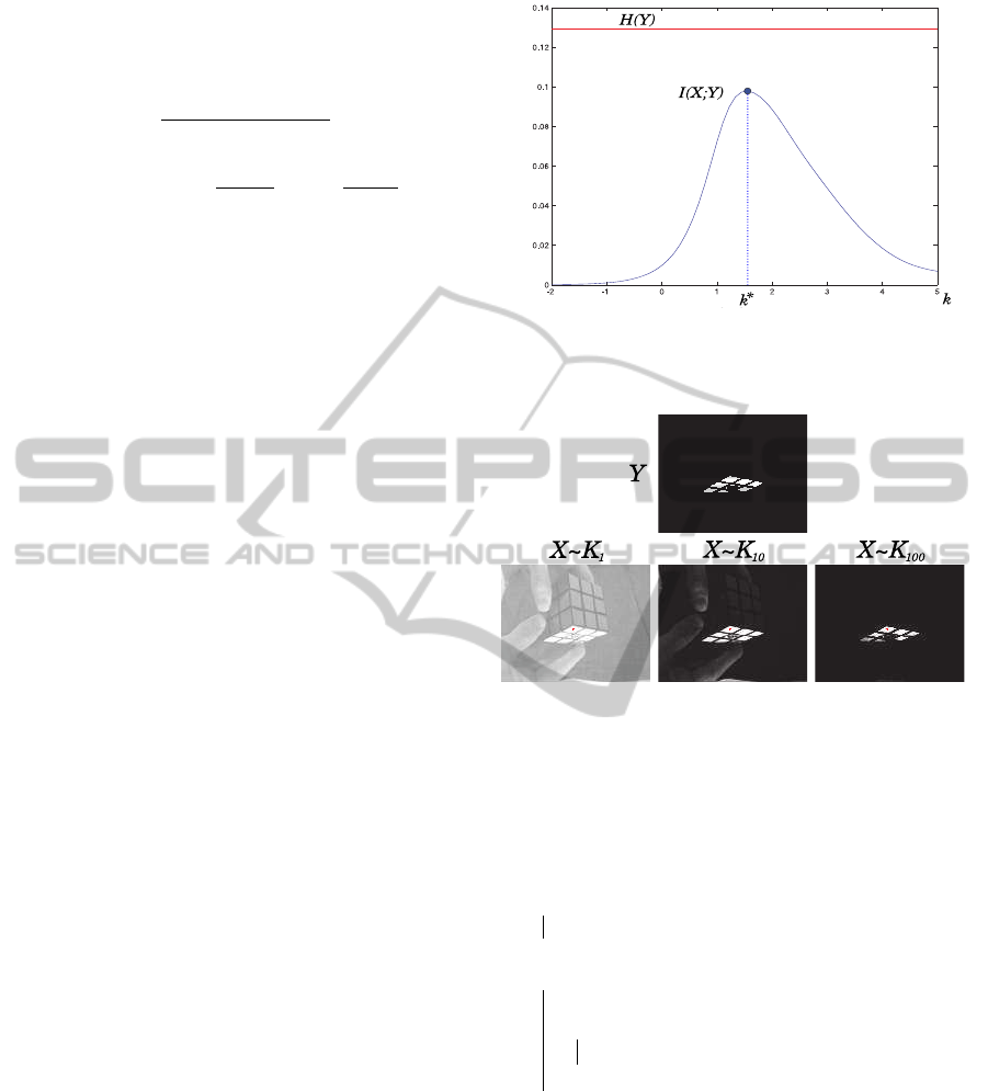
The parameter λ is very important. We optimize it
by maximizing the mutual information I between the
probability map X and the labels Y (MacKay, 2003):
I(X;Y) = H(X) + H(Y) − H(X,Y)
This optimization via, for example, the
Levenberg-Marquardt method quickly converges
to a solution λ
∗
. We do not detail it and simply
present a possible evolution of I depending on λ in
Figure 2.
Figure 3 shows the evolution of X from white to
black depending on the kernel bandwidth λ. When
λ becomes small the map of probabilities becomes all
white ( lim
λ→0
+
e
−λ.d
= 1) and the informationexchanged
with the labels null. When λ becomes large the prob-
ability map is all black ( lim
λ→+∞
e
−λ.d
= 0) and mutual
information null again. Between the two there is a λ
∗
solution as 0 ≤ I(λ
∗
) ≤ H(Y).
2.2 Kernel Selection
N = 9M kernels, optimal in the sense of λ, were gen-
erated but only K with K ≪ N are selected. The goal
is to keep the set the most representative of the labels
Figure 2: Kernel bandwidth optimization by maximizing
the mutual information with the labels Y. I = f(λ) with
λ = 10
k
where k = [-2, 5].
Figure 3: Evolution of the map of probabilities X based on
the kernel bandwidth. Y vs X for λ = {1, 10, 100}.
Y of the ROI of the first image. This was performed
by the CMIM algorithm (Conditional Mutual Infor-
mation Maximization) (Fleuret, 2004) with a novelty
to compare booleans to probabilities:
for n=1...N do
s[n] ← I(Y;X
n
)
end
for k=1...K do
ν[k] = arg max
n
s[n]
for n=1...N do
s[n] ← min{s[n], I(Y;X
n
|X
ν[k]
)}
end
end
Algorithm 1: CMIM algorithm.
I(Y;X
n
|X
m
) =H(Y,X
m
) − H(X
m
)
− H(Y,X
n
,X
m
) + H(X
n
,X
m
)
For the calculations of H(X
n
,X
m
) and
H(Y,X
n
,X
m
) the labels Y and the probability
maps X
n
and X
m
are assumed to get as much
information as possible together. For instance,
for one pixel, if p
n
= 0.8 and p
m
= 0.7 then
VISAPP 2012 - International Conference on Computer Vision Theory and Applications
374
p
(X
n
=1)∩(X
m
=1)
= min(p
n
, p
m
) = 0.7. This exchange
of information can be represented by a noisy channel
with H(X
n
) ≤ H(X
m
).
Figure 4 shows an example of the selection of five
kernels by CMIM based on Figure 1:
[19, 9] XY
[ 8,24] B [18, 4] G [26, 3] XY [ 1, 9] B
Figure 4: Selection of 5 kernels by CMIM.
2.3 k-PPV MCMC Tracking
The goal is to find in each new image the closest
ROI to the original. Information is normalized by
dimension and weighted on UVRGB by the weights
[1/4, 1/4, 1/6, 1/6, 1/6]. Each image can be viewed
as a probability density function (PDF) and compared
with another one by a similarity measure, namely
the Kullback-Leibler divergence. (Boltz et al., 2009)
showed how to estimate it in a k-NN framework and
why it is well aware of the local densities in high di-
mensions.
For a reference population R of n
R
points in di-
mension d and a target population T of n
T
points in
the same dimension (n
R
6= n
T
a priori), with ρ
k
(U, s),
the Euclidean distance between the point s and its k
th
nearest neighbor in U (U ≡ R or T), the Kullback-
Leibler divergence D
KL
(T,R) can be estimated, in an
unbiased way, by:
D
KL
(T,R)
kPPV
= log
n
R
n
T
− 1
+
d
n
T
∑
s∈T
log
ρ
k
(R,s)
ρ
k
(T,s)
An ideal estimation would consider all the pixels
of R and T. However, to avoid the combinatorial ex-
plosion or just speed up the calculations, we try to
downsample these regions. The question is how. We
have compared three types of sub-samples: two regu-
lar, one random and one from the kernels selected by
CMIM.
Trackings use a sequential particle filter (Arulam-
palam et al., 2002) with a Markov chain (Khan et al.,
2005). Each particle represents a region of the im-
age. The upper left corner of the reference ROI R
indicates the first position. From the second we ap-
ply N
p
random transformations ϕ
i
to R. It gener-
ates N
p
particles or ROI targets T
i
whose weight is:
w
i
= e
−µ.D
KL
(T
i
,R)
with µ a fixed constant. The parti-
cle with the maximum weight takes on the new posi-
tion. The others are not forgotten. They will generate
new particles in the subsequent iterations. The repro-
duction rate is governed by the Metropolis-Hastings
rule: min(1,w
new
/w
∗
) < rand(). Few particles of low
weight are also ”burned” at each iteration.
We have also several important assumptions: that
the reference R doesn’t not change, that the object is
far from the camera and therefore that the ROI under-
goes only translations and remains fixed.
3 EXPERIMENTS
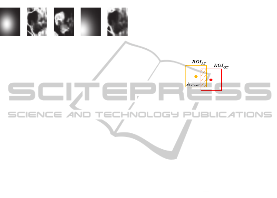
A manual tracking provided the ground truth GT. The
particle filter algorithm truth AT was then compared
to GT following different configurations.
Figure 5: Intersection area A
AT∩GT
of the ROI of the algo-
rithm AT and of the ground truth GT in the same image.
To determine the quality η of a tracking, AT and
GT were compared image by image. We calculated
their reports of intersection area and union area and
check whether for a given tolerance τ it makes ”fit”
the tracked ROIs to the ground truth or not. This state,
good or not, is rated β. For N
i
images:
β
i
(τ) =
(
1 if
A
i
AT∩GT
A
i
AT∪GT
≥ τ
0 else
η(τ) =
1
N
i
N
i
∑
i=1
β
i
(τ)
Four significant subsamplings are presented: reg-
ular on raw data (”Raw”), regular on data smoothed
by a Gaussian kernel (”Gauss”), random on data aver-
aged per Voronoi cell (”RandVor”), and finally from
the convolution of kernels selected by CMIM with
their optimized bandwidth (”KerOpt”).
Results are based on the sequence ”Walk-
ByShop1cor” of CAVIAR between images 192 and
309. We tried to follow the head of a man on a win-
dow of size 31× 25 pixels. The curves show the vari-
ation of good tracking η depending on the tolerance
τ on the percentage of area common with the ground
truth. The four curves in green, khaki, brown and red
in Figure 6 represent subsamplings of a pixel of 1, 4,
7 and 10 i.e.: 775, 56, 20 and 12 points for the con-
figurations ”Raw”, ”Gauss” and ”RandVor”, from top
to bottom. Down on the same figure, the three curves
gray, violet and cherry compile the ”KerOpt” config-
uration for respectively: 55, 30 and 5 points filtered
from the selected kernels.
KERNEL SELECTION BY MUTUAL INFORMATION FOR NONPARAMETRIC OBJECT TRACKING
375
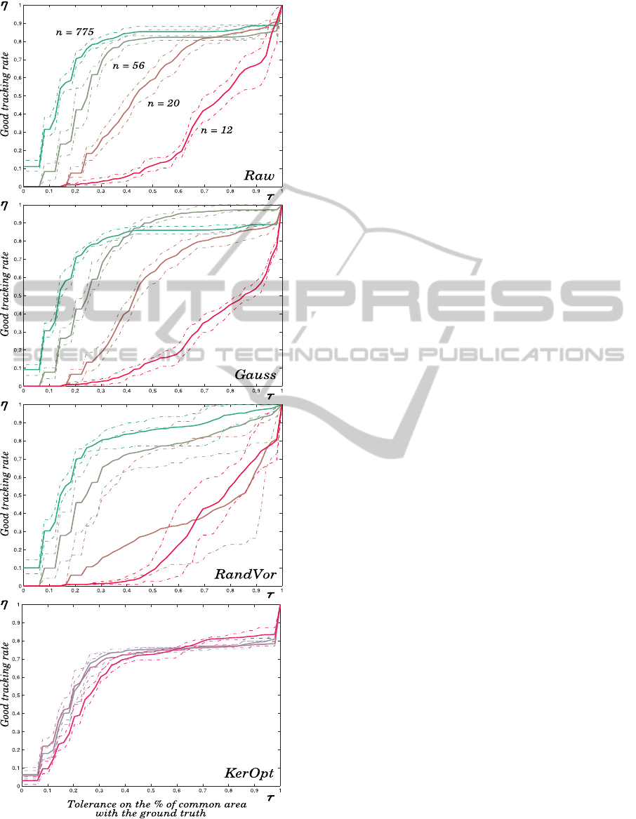
Figure 6: Tracking performances η(τ) of the subsamplings
”Raw”, ”Gauss” and ”RandVor” for K = {775, 56, 20, 12}
points and ”KerOpt” for K = {55, 30, 5} points.
4 CONCLUSIONS
Our goal was to track a target with appearance model
at low cost, i.e. based on few points. We have shown
how to build a light model made up of independent
and representative kernels of the prime appearance.
Trackings made with this filtering were compared to
other more traditional and showed equivalent perfor-
mance for a number of points lower.
However, many things has to be improved. Here’s
a partial list: 1) integrate the temporal coherence in
addition to the spatial coherence by introducing ex-
plicit time T in a new representation, for instance:
UVRGBT, 2) make evolve the reference ROI R along
the tracking by an on-line learning of new likely la-
bels, 3) add new parameters to the transformation ϕ
to consider rotations or homotheties or even why not
see ϕ in a nonparametric way by considering each
point of the model as a single control point connected
to other by a consistent deformable mesh. All these
points seem difficult but not unattainable.
REFERENCES
Arulampalam, M., Maskell, S., Gordon, N., and Clapp,
T. (2002). A tutorial on particle filters for on-
line nonlinear/non-gaussian bayesian tracking. Signal
Processing, IEEE Transactions on, 50(2):174–188.
Boltz, S., Debreuve, E., and Barlaud, M. (2009). High-
dimensional statistical measure for region-of-interest
tracking. IEEE Transactions on Image Processing,
18(6):1266–1283.
Comaniciu, D., Ramesh, V., and Meer, P. (2000). Real-
time tracking of non-rigid objects using mean shift.
In CVPR, volume 2, pages 142–149. Published by the
IEEE Computer Society.
Fleuret, F. (2004). Fast binary feature selection with con-
ditional mutual information. The Journal of Machine
Learning Research, 5:1531–1555.
Fukunaga, K. and Hostetler, L. (1975). The estimation of
the gradient of a density function, with applications in
pattern recognition. IEEE Transactions on Informa-
tion Theory, 21(1):32–40.
Garcia, V., Debreuve, E., and Barlaud, M. (2008). Fast k
nearest neighbor search using GPU. In CVPR Work-
shop on Computer Vision on GPU (CVGPU), Anchor-
age, Alaska, USA.
Khan, Z., Balch, T., and Dellaert, F. (2005). Mcmc-based
particle filtering for tracking a variable number of in-
teracting targets. IEEE Transactions on Pattern Anal-
ysis and Machine Intelligence, pages 1805–1918.
MacKay, D. (2003). Information theory, inference, and
learning algorithms. Cambridge University Press.
Parzen, E. (1962). On the estimation of a probability den-
sity function and mode. The Annals of Mathematical
Statistics, 33(3):1065–1076.
VISAPP 2012 - International Conference on Computer Vision Theory and Applications
376
