OPTIMAL CONTROL THEORY FOR MULTI-RESOLUTION
PROBLEMS IN COMPUTER VISION
Application to Optical-flow Estimation
Pascal Zille
1,2
and Thomas Corpetti
2
1
UMR CNRS LMFA, Ecole Centrale Lyon, Lyon, France
2
CNRS LIAMA TIPE, Beijing, China
Keywords:
Multi-resolution, Optical-flow, Optimal Control, Data Assimilation.
Abstract:
This paper is concerned with the multi-resolution issue used in many computer vision applications. Such ap-
proaches are very popular to optimize a cost function that, in most of the situations, has been linearized for
mathematical facility reasons. In general, a multi-resolution setup consists in a redefinition of the problem at
a different resolution level where the mathematical assumptions (usually linearity) hold. Following a coarse-
to-fine strategy, a usual process consists in 1) optimizing the large scales and 2) use this result as an initial
condition for the estimation at finer scales. Such process is repeated until the plain image resolution. One
of the main drawbacks of such downscaling approach is its incapacity to correct the eventual errors that have
been made at larger scales. These latter are indeed propagated along the scales and disturb the final result.
In this paper, we suggest a new formulation of the multi-resolution setup where we exploit some smoothing
techniques issued from optimal control theory and in particular variational data assimilation. The time is here
artificial and is related to the various scales we are dealing with. Following a consistent mathematical frame-
work, we define an original downscaling/upscaling technique to perform the multi-resolution. We validate this
approach by defining a simple optical flow estimation technique based on Lucas-Kanade. Experimental results
on synthetic data demonstrate the efficiency of this new methodology.
1 INTRODUCTION
A number of common computer vision techniques
(related to motion estimation, segmentation, charac-
terization, ...) are defined as finding a variable X by
solving an equation H (X,I, X
X
X
0
) that depends on the
image luminance I and the pixel grid X
X
X
0
(also noted x
x
x
in this paper). Because most of the usual assumptions
hold only in a linear case for obvious mathematical
properties, it is common to embed the resolution of
H (X,I,X
X
X
0
) in a so-called “multi-resolution” scheme
(Burt, 1988; Mallat, 1989). The main principle con-
sists in redefining the images on smaller grids X
X
X
N
that
correspond to the initial grid X
X
X
0
divided by a factor
N. On such “coarse” images, we assume that de res-
olution of H (X,I,X
X
X
N
) can be done under linear con-
straints and this provide a coarse approximation X
N
of the final solution X. In a step forward, this approx-
imation X
N
is used as an initial condition for a new
problem where the goal is to extract a refinement dX
(with X = X
N
+ dX) that can be estimated from X
N
using linear constraints. Such process is commonly
repeated for several levels of resolutions, yielding a
succession of linear problems.
This is for instance a usual way to deal with
optical-flow estimation where the common bright-
ness consistencyassumption (that links the spatial and
temporal gradients of the luminance with the spatial
velocity v
v
v(x
x
x) to estimate), defined as:
∂I
∂t
+ v
v
v(x
x
x) ·∇I ≈ 0 (1)
holds only for small displacements. When embedded
in a multi-resolution scheme, this relation holds for
the images at the coarser resolutions and the associ-
ated estimations are used as initial solutions for the
finer resolutions.
To get such “coarse” data on which the problem
is solved, a usual strategy consists in using a pyra-
midal decomposition of the images, for instance with
wavelet decompositionsor gaussian filtering followed
by decimations, as illustrated in FIG. 1(left) for a fac-
tor N = 2. The estimation is then performed first from
the smallest images (under linear constraints) and the
134
Zille P. and Corpetti T..
OPTIMAL CONTROL THEORY FOR MULTI-RESOLUTION PROBLEMS IN COMPUTER VISION - Application to Optical-flow Estimation.
DOI: 10.5220/0003841401340143
In Proceedings of the International Conference on Computer Vision Theory and Applications (VISAPP-2012), pages 134-143
ISBN: 978-989-8565-04-4
Copyright
c
 2012 SCITEPRESS (Science and Technology Publications, Lda.)

Solution 1 :
Filtering + decimation
Solution 2 :
Gaussian smoothings
grid X
X
X
0
grid X
X
X
ℓ
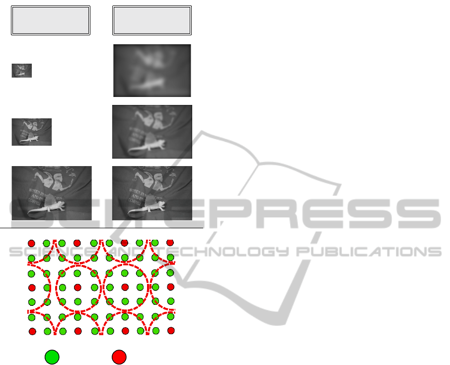
Figure 1: Multiresolution strategies. Top left: classical
pyramidal decomposition; top right: successive gaussian
convolutions. Bottom: illustration of the latter technique.
Green circles represent the original pixel grid whereas the
red ones represent the grid at a given resolution ℓ.
solution is reprojected to the following level. Another
possibility proposed in (Corpetti and M´emin, 2012)
consists in obtaining X
ℓ
(related to the solution of a
problem H (X,I, X
X
X
ℓ
) at a resolution ℓ) by perform-
ing a convolution of H (X,I, X
X
X
0
) by a gaussian ker-
nel of standard deviation ℓ. Indeed, a multi-resolution
scheme consists in redefining the problem on a grid
X
X
X
ℓ
which can be viewed as a coarse representation of
the initial grid X
X
X
0
= X
X
X with a Brownian isotropic un-
certainty of constant variance ℓ :
X
X
X
ℓ
= X
X
X
0
+ ℓ I
2
dB
B
B, (2)
where B
B
B is a standard Brownian motion and I the
2D identity matrix (see the illustration in figure 1).
Under this scheme, any solution X
ℓ
of a problem
H (X,I,X
X
X
ℓ
) defined on a grid X
X
X
ℓ
should satisfy the
expectation E(H (X,I, X
X
X
ℓ
)|X
X
X
0
) which is equivalent
(see (Corpetti and M´emin, 2012) for the demon-
stration) to a convolution of H (X,I, X
X
X
0
) with the
isotropic centered gaussian N (0,ℓ) of variance ℓ.
Therefore the multi-resolution can be performed
by solving a family of problems g
ℓ
∗ H (X,I, X
X
X
0
)
at the various resolutions ℓ. A main advantage of
such a formulation of the multi-resolution setup is to
naturally get rid of the intrinsic problems related to
pyramidal image decompositions (decimations and
interpolations in particular). In addition, instead of
dealing with successive decimations of factor 2 of
the initial image to fix the different multiresolution
levels, the evolutions of the levels ℓ are much flexible
here.
General difficulties of multi-resolution sys-
tems: even if several specific techniques have been
proposed for some applications (see for instance
(Alvarez et al., 2000; Baatz and Schaape, 2000;
Bajcsy and Kovacic, 1989; Brox et al., 2004; Eck
et al., 1995; Ojala et al., 2002)), in general, whatever
the multi-resolution setup chosen, one of the main
difficulty remains on the succession of independent
problems: at a given resolution ℓ
n
, the problem
consists in finding dX
ℓ
n
using X
ℓ
n+1
as a coarse
approximation: X
ℓ
n
= X
ℓ
n+1
+ dX
ℓ
n
. Once X
ℓ
n
estimated, its value is kept during the rest of the
process. This is somewhat prejudicial since it is
now recognized that small scales (related to finer
resolutions) interact with larger scales. With such
schemes, at a given resolution ℓ
n
, the information
related to smaller scales ℓ < ℓ
n
can not be taken
into account. In addition, any error in the estimation
of X
ℓ
n
will also be kept and propagated across the
resolutions without any possibilities of correction.
To deal with these difficulties, we propose in
this paper an original solution based on optimal con-
trol theory and in particular on data assimilation.
Such schemes consist in estimating a sequence of un-
knowns X(t) driven by a more or less exact dynamical
model by performinga series of forward/backward in-
tegrations. The key idea of this study is to exploit
such framework where the time will in fact be related
to the various scales. The forward/backward integra-
tions will then lead to a set of upscaling/downscaling
approaches that appear to be adapted to our problem.
Before entering into the core of the technique in sec-
tion 3, we first briefly introduce the data assimilation
framework.
2 DATA ASSIMILATION
In this section we will describe the general principles
OPTIMAL CONTROL THEORY FOR MULTI-RESOLUTION PROBLEMS IN COMPUTER VISION - Application to
Optical-flow Estimation
135

of the assimilation scheme we devised in this study.
Variational data assimilation is a technique derived
from optimal control theory (Lions, 1971) to recover
a state variable’s trajectory from a sequence of mea-
surements. Opposite to sequential Bayesian filters,
which share the same aim, this framework allows
to handle high dimensional systems (and is thus in-
tensively used for instance in environmental sciences
(Bennett, 1992; Le Dimet and Talagrand, 1986; Ta-
lagrand and Courtier, 1987)). We refer the reader to
(Bennett, 1992; Le Dimet and Talagrand, 1986; Li-
ons, 1971; Talagrand and Courtier, 1987; Talagrand,
1997; Vidard et al., 2000) for complete methodologi-
cal aspects of data assimilation and applications con-
cerning geophysical flows.
The problem consists in recovering, from an ini-
tial condition X
0
, a system’s state X partially observed
and driven by approximately known dynamics. This
can be formalized as finding X(x
x
x,t), for any location
x
x
x ∈ Ω at time t ∈ [t
0
,t
f
], that satisfies the system:
∂X
∂t
(x
x
x,t) + M(X(x
x
x,t)) = ν
m
(x
x
x), (3)
X(x
x
x,t
0
) = X
0
(x
x
x) + ν
n
(x
x
x), (4)
Y
Y
Y(x
x
x,t) = H(X(x
x
x,t)) + ν
o
(x
x
x,t), (5)
where M is the non-linear operator relative to the dy-
namics, X
0
is the initial vector at time t
0
and (ν
n
,ν
m
)
are (unknown) additive control variables relative to
noise on the dynamics and the initial condition re-
spectively. In addition, noisy measurements Y
Y
Y of the
unknown state are available through the non-linear
operator H, up to ν
o
. To estimate the system’s state,
a common methodology relies on the minimization of
the cost function J :
J (X) =
1
2
Z
t
f
t
0
kY
Y
Y −H(X(ν
m
,ν
n
))k
2
R
−1
dt
+
1
2
kX(x
x
x,t
0
) −X
0
(x
x
x)k
2
B
−1
+
1
2
Z
t
f
t
0
k
∂X
∂t
(x
x
x,t) + M(X(x
x
x,t))k
2
Q
−1
dt,
(6)
where we have introduced the information matri-
ces R,B,Q relative to the covariance of the errors
(ν
m
,ν
n
,ν
o
). The Mahalanobis distance that has been
used reads, for an information matrix A: kXk
A
−1
=
X
T
A
−1
X. The evaluation of X can be done by can-
celing the gradient δJ
X
(θ) = lim
β→0
J(X+βθ)−J(X)
β
of
(6). Unfortunately, the estimation of such gradient is
in practice unfeasible for a large system’s state since it
would be necessary to integrate the dynamical model
along all possible perturbations of the components of
X. This is computationally impossible with actual
hardwares when one deals with a complete sequence
of images and complex dynamical models. One way
to cope with this difficulty is to write an adjoint for-
mulation of the problem. To that end, the adjoint vari-
ables λ
λ
λ that express the errors of the dynamic model
are introduced as:
λ
λ
λ(x
x
x,t) =
Z
Ω,t
Q
−1

∂X
∂t
+ M(X)

dx
′
dt
′
(7)
Denoting:
•

∂M
∂
e
X

and

∂H
∂
e
X

the linear tangent operators of
M and H respectively. The linear tangent of an
operator A is the directional derivative of the op-
erator (the Gˆateaux derivative):

∂A
∂
e
X

(dX) = lim
β→0
A(
e
X + βdX) −A(
e
X)
β
, (8)
• (∂
X
M)
∗
and (∂
X
H)
∗
their adjoint operators. The
adjoint A
∗
of a linear operator A on a space D is
such as:
∀x
1
,x
2
∈ D ,< Ax
1
,x
2
>=< x
1
,A
∗
x
2
>, (9)
it can be shown that canceling the gradient δJ
X
(θ)
with respect to the adjoint variables λ
λ
λ leads to a ret-
rograde integration of an adjoint evolution model that
takes into account the observations. Once the adjoint
variables λ
λ
λ are estimated, one can recover the system
state X using relation (7). Finally, when dealing with
non-linear models, recovering X leads to the follow-
ing incremental algorithm (Bennett, 1992):
1. Starting from
˜
X(x
x
x,t
0
) = X
0
(x
x
x), perform a forward inte-
gration:
∂
˜
X
∂t
+ M(
˜
X) = 0
2.
˜
X(x
x
x,t) being available, compute the adjoint vari-
ables λ
λ
λ(x
x
x,t) with the backward equation:
λ
λ
λ(t
f
) = 0 ;
−
∂λ
λ
λ
∂t
(t) + (∂
X
M)
∗
λ
λ
λ(t) = (∂
X
H)
∗
R
−1
(Y
Y
Y −H(
˜
X))(t)
(10)
3. Update the initial condition : dX(t
0
) = Bλ
λ
λ(t
0
);
4. λ
λ
λ being available, compute the state space dX(t) from
dX(t
0
) with the forward integration
∂dX
∂t
(t) +

∂M
∂
˜
X

dX(t) = Qλ
λ
λ(t) (11)
5. Update :
˜
X =
˜
X +dX
6. Loop to step (2) until convergence
Intuitively, the adjoint variables λ
λ
λ contain infor-
mation about the discrepancy between the observa-
tions and the dynamic model. They are computed
from a current solution
˜
X with the backward integra-
tion (10) that encompasses both the observations and
the dynamic operators. This deviation indicator be-
tween the observations and the model is then used to
VISAPP 2012 - International Conference on Computer Vision Theory and Applications
136

refine the initial condition (step (3)) and to recover
the system state through an imperfect dynamic model
where errors are Qλ
λ
λ (step (4)). It should be noted
that if the dynamic is perfect, the associated error co-
variance Q is zero and the algorithm only refines the
initial condition.
Graphic Illustration of the Incremental Algo-
rithm. Let us try to illustrate in a simple way ’what
is the algorithm doing’. For the sake of clarity, we
will consider here the case of a prefect dynamic model
where only the initial condition is refined.
-Let’s take a closer look at (step (1)) of the abovemen-
tionned algorithm: it consists in determining a first
coarse ’trajectory’ of X. As shown in figure 2(a), we
start from an initial condition X(t
0
) and compute the
state variable values ∀t ∈ [t
0
,t
f
] using a forward in-
tegration of the dynamical model M. The red circles
symbolically represent the available measurementsY
Y
Y.
-Having a first estimation of X, we may now move on
to (step (2)), ie solving the backward integration that
encompasses both the observations and the dynamic
operators. As represented in figure 2(b), this step con-
sists in integrating from t
f
to t
0
the adjoint dynamic
model (10) and may be understood as a backpropaga-
tion of the discrepancy between our estimated trajec-
tory and the observations Y
Y
Y.
-The purpose of computing the adjoint variable is to
use its initial value λ
λ
λ(t
0
) and the relation defined in
(step (3)), thus obtaining an initial increment dX(t
0
).
We then aim at ’propagating’ this latter along the time
axis integrating forward the tangent model (11).
-Finally, updating the previous estimation with this
increment should yield a better compromise between
the dynamical model and the observations, figure 2(c)
Remarks on Variationnal Assimilation. An inter-
resting property of variationnal assimilation is the
mutual interraction of all estimations. That is for each
(t
1
,t
2
) ∈[t
0
,t
f
]
2
the estimated value of X(t
1
) at a given
iteration can influence the value of X(t
2
) and vice
versa. This yields to more coherent estimation than
sequential assimilation where values of X for a given
time t
∗
may only interract with values for t > t
∗
. This
framework is then an appealing solution for large sys-
tem states and acts as a smoothing issue. To design an
assimilation process, we need to define:
1. The system state;
2. The dynamical model (and its adjoint);
3. The observation operator (and its adjoint);
4. The error covariance matrices.
In this paper, we suggest to exploit this framework
for defining an original multi-resolution system. The
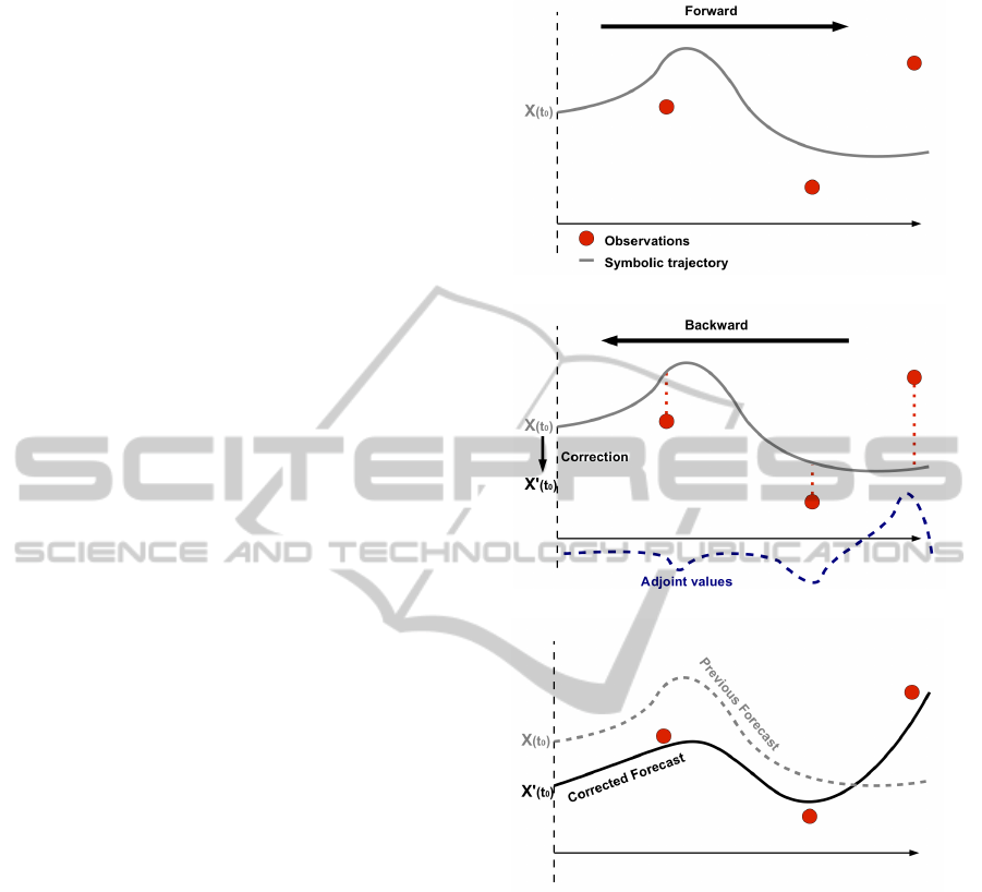
(a) forward integration starting from inital condition (step (1))
(b) backward adjoint integration and initial correction (steps (2)-(3))
(c) forward tangent integration and correction propagation (steps (4)-(5))
Figure 2: Symbolic illustration of one iteration of the incre-
mental algorithm.
temporal variable will be related to the spatial scales,
as presented in the next section.
3 VARIATIONAL ASSIMILATION
FOR MULTI-RESOLUTION
Unlike most of existing issues related to variational
assimilation, in this article the usual temporal variable
t is now connected to the different resolutions. To
avoid ambiguities, we then rather prefer to represent
its value with the scale parameter ℓ. A value ℓ = 0
corresponds to the “plain” resolution at the image grid
OPTIMAL CONTROL THEORY FOR MULTI-RESOLUTION PROBLEMS IN COMPUTER VISION - Application to
Optical-flow Estimation
137

(ℓ = 0 ⇒ grid X
X
X
0
= x
x
x) and we assume that the system
state X evolves across the resolutions following scale
space relation:
∂X
∂ℓ
=
1
2
∆X. (12)
Indeed, it can easily be demonstrated that the solution
of the previous relation is
X
ℓ
= X(ℓ) = g
√
ℓ
∗X(0), (13)
where g
√
ℓ
is a gaussian kernel of standard devia-
tion ℓ. As shown in section 1, this relation enables
to access the various scales of X. The linear model
M(X) = −
1
2
∆X associated to relation (3) and corre-
sponding to the scale space evolution (12) is then a
perfect model for an exploration of X at different res-
olution levels. We then suggest to rely on this re-
lation, using the assimilation framework of the pre-
vious section, to define a multi-resolution system.
Following the definition of adjoint operators, we get
(∂
X
M)
∗
(X) = M(X) = −
1
2
∆X.
The new multi-resolution procedure consists now
to estimate X(0) at the initial artificial time ℓ = 0
(which corresponds to the image grid) under the per-
fect model of relation (12). The initial condition X
0
is set to zero and the observation system Y
Y
Y(X
X
X
0
) =
H(X
X
X
0
,X
0
) defined at the image grid X
X
X
0
reads for any
resolution ℓ > 0 :
(
Y
Y
Y(X
X
X
ℓ
) = g
√
ℓ
∗Y
Y
Y(X
X
X
0
)
H(X
X
X
ℓ
,X
ℓ
) = g
√
ℓ
∗H(X
X
X
0
,X
0
).
(14)
Following the algorithm described in section 2, as the
first integration of the dynamic model in (12) with
null initial condition gives zeros for all ℓ, the process
is expressed as (with B and R the error covariance ma-
trices related to the uncertainty on the initial condition
and the observations):
• Initialization:
˜
X(ℓ) = 0 for all scales ℓ ∈ [0, ℓ
f
].
1. Compute the adjoint variables λ
λ
λ(ℓ) with the downscal-
ing equation:
λ
λ
λ(ℓ
f
) = 0 ;
−
∂λ
λ
λ
∂ℓ
(ℓ) −
1
2
∆λ
λ
λ(ℓ) =

∂
X
H
ℓ

∗
R
−1
(Y
Y
Y(X
X
X
ℓ
) −H(X
X
X
ℓ
,
˜
X
ℓ
))
(15)
2. Adjoint variables λ
λ
λ being available, update the correc-
tion at the image grid : dX(0) = Bλ
λ
λ(0);
3. Assess to the correction at all the resolution levels dX(ℓ)
from dX(0) with the upscaling equation:
∂dX
∂ℓ
=
1
2
∆dX (16)
4. Update :
˜
X =
˜
X +dX, ∀ℓ ∈ [0,ℓ
f
]
5. Loop to step (1) until convergence
Comments of the new multi-resolution scheme: the
first step of the previous algorithm corresponds to the
usual downscaling approach: from coarse to fine res-
olutions, we compute and propagate the errors with
equation (15). This enables to refine the solution at
the image grid (step 2). Unlike the classic multi-
resolution approach which ends here, we then re-
propagate this correction at the various resolutions
(step 3). The process is then repeated until conver-
gence. This framework enables to modify former so-
lutions at given resolution ℓ = L by taking into ac-
count their influence on smaller scales ℓ < L. This
answers a difficulty mentioned in section 1 and au-
thorizes a correction of the estimations at all the res-
olution levels. As the dynamical model is perfect, for
each application we need to define an observationsys-
tem Y
Y
Y(X
X
X
ℓ
) = H(X
X
X
ℓ
,X
ℓ
), its associated error covari-
ance matrix R and the one related to the null initial
condition B. In the next section, we apply this frame-
work for optical-flow estimation.
4 APPLICATION TO
OPTICAL-FLOW
The goal of this section is to demonstrate the effi-
ciency of the introduced multi-resolution procedure.
To that end, we use the context of optical flow estima-
tion and we compare results reached using two classic
and our new multi-resolution approaches.
The optical-flow problem consists in estimating a
velocity field X(x
x
x) = v
v
v(x
x
x) = [u(x
x
x),v(x
x
x)]
T
at the image
grid x
x
x between two images I
1
(x
x
x) and I
2
(x
x
x).
As mentioned above, the framework of section 3
is valid for any kind of applications, depending on
the observation operator H. In this example related
to motion estimation, we use a simple Lucas-Kanade,
presented in the next paragraph. It should be outlined
that this observation model is implemented for a test-
ing issue but obviously, one of the main advantage
of this framework is its possibility to naturally embed
in the observation term more advances techniques, as
continuity preserving ones or some physical models
accurately defined at a given resolution ℓ (sub-grid
models in particular).
4.1 Observation Operator based on
Lucas-Kanade
The most used and simple observation model pro-
posed for optical-flow estimation is the brightness
consistency assumption:
dI
dt
=
∂I(x
x
x,t)
∂t
+ v
v
v(x
x
x,t) ·∇I(x
x
x,t) ∼ 0 (17)
VISAPP 2012 - International Conference on Computer Vision Theory and Applications
138

and assumes that the points x
x
x keep their inten-
sity along their displacements, the luminance I
being viewed as a continuous function and ∇ =
(∂/∂x,∂/∂y)
T
being the gradient operator. Applied
to a pair of images this relation reads:
I
2
(x
x
x+ ∆tv
v
v(x
x
x)) −I
1
(x
x
x) = 0 ⇒
I
2
(x
x
x) −I
1
(x
x
x)
∆t
+ v
v
v(x
x
x) ·∇I
2
(x
x
x) = 0
(18)
where we have a first order Taylor development of
the conservation constraint I
2
(x
x
x+ ∆tv
v
v(x
x
x))−I
1
(x
x
x) = 0
around ∆tv
v
v(x
x
x) and ∆t is the time between two im-
ages (by convention we assume ∆t = 1). This cre-
ates a link between the displaced frame difference
I
2
(x
x
x) −I
1
(x
x
x), the spatial gradients of the second im-
age ∇I
2
(x
x
x) and the velocity v
v
v to estimate. The equa-
tions in (17-18) are commonly named the optical-flow
constraint equations (OFCE) and are the basis of huge
amount of studies. The reader can refer to (Baker
and Matthews, 2004; Baker et al., 2007; Baker et al.,
2010; Barron et al., 1994; Galvin et al., 1998; Mitiche
and Bouthemy, 1996) for presentations and overviews
of optical flow techniques. At this step, it is easy to
observe that:
1. in homogeneous areas, all terms vanish and there
is an infinity of solutions;
2. because of the projection v
v
v ·∇I, only the normal
component to the photometric gradients can be
extracted with such a formulation. This problem
is known as the “aperture problem”.
Therefore, the relations in (17-18) are in themselves
not sufficient to extract the velocity field. We need to
add some constraints on the velocity to estimate.
In the work of Lucas & Kanade (Lucas and
Kanade, 1981), the authors have assumed for each lo-
cation x
x
x that the velocity is locally constant. It is then
estimated as:
v
v
v = min
v
v
v=(u,v)
T
Z
Ω
g
σ
∗

∂I(x
x
x,t)
∂t
+ v
v
v(x
x
x,t) ·∇I(x
x
x,t)

2
dx
x
x,
(19)
where g
σ
is a Gaussian window of standard deviation
σ in which the velocity v
v
v is assumed to be homoge-
neous. Canceling the derivative of the previous rela-
tion with respect to v
v
v leads to:
v
v
v = −

g
σ
∗

I
2
x
I
x
I
y
I
x
I
y
I
2
y

−1
g
σ
∗

I
x
I
t
I
y
I
t

, (20)
where I
•
= ∂I/∂•. To guarantee a good condition-
ing of the previous matrix to invert, the spatial gradi-
ents must not vanish. The gaussian smoothing aims
in fact at alleviating homogeneous areas by capturing
the spatial information at a scale related to σ. On the
basis of relation (20), we then define our observation
system where the unknown X
ℓ
can be set at each res-
olution X
X
X
ℓ
with the linear Lucas-Kanade based obser-
vation system Y
Y
Y(X
X
X
ℓ
) = H(X
X
X
ℓ
)X
ℓ
as:







Y
Y
Y(X
X
X
ℓ
) = g
√
ℓ
∗g
σ
∗

I
x
I
t
I
y
I
t

H(X
X
X
ℓ
) = −g
√
ℓ
∗

g
σ
∗

I
2
x
I
x
I
y
I
x
I
y
I
2
y

.
(21)
The adjoint operator of H is itself and g
σ
is a convo-
lution with a gaussian of standard deviation σ related
to the Lucas & Kanade strategy.
4.2 Error Covariance Matrix and
Initialization Issues
Error covariance matrix related to the observation:
we have defined, at each point of the grids X
X
X
ℓ
, the
matrix R
−1
used in (10) as a diagonal one such that:
R
−1
(X
X
X
ℓ
) = R
max
exp−
[Y
Y
Y(X
X
X
ℓ
) −H(X
X
X
ℓ
)]
2
σ
2
obs
(22)
As shown in (Corpetti et al., 2009), this penalization
amounts to consider a robust norm in relation (19).
Such a robust function allows the discarding of points
having large “residual” values of the observation
error [Y
Y
Y(X
X
X
ℓ
) − H(X
X
X
ℓ
)] (called outliers in the Ro-
bust Statistics literature (Huber, 1981; Geman and
Reynolds, 1992; Delanay and Bresler, 1998)). In our
application, it enables to properly deal with corrupted
areas that do not fit our data model exactly.
Initial conditions: as mentioned in section 3,
we have no prior knowledge X
0
. We then have set
X
0
= 0. Therefore the associated covariance matrix B
is
B(X
X
X
0
) = Id −exp

−|I
2
(X
X
X
0
) −I
1
(X
X
X
0
)|
2
/σ
2
B

(23)
where σ
B
is a parameter to fix. It is related to the
adequacy of the null solution depending on the OFCE.
Complete scheme: the multi-resolution strategy
of section 3 with the observation operator defined
in (21) and the associated error covariance matrixes
R and B (defined in (22) and (23) respectively)
constitute the complete framework for optical-flow
estimation using an original downscaling/upscaling
multi-resolution process. Let us now turn to some
experimental results.
OPTIMAL CONTROL THEORY FOR MULTI-RESOLUTION PROBLEMS IN COMPUTER VISION - Application to
Optical-flow Estimation
139

Table 1: Quantitative comparisons on the DNS sequence with a Pyramidal Lucas-Kanade (LK, (Lucas and Kanade, 1981)),
a Lucas-Kanade term embed in a multi-resolution scheme with successive convolutions without any assimilation (CONV)
and the proposed multi-resolution using variational assimilation (AMR). In addition, we have plotted numerical values issued
from a commercial technique based on correlation (COM, LA VISION SYSTEM), Horn & Schunck (HS, (Horn and Schunck,
1981)), two fluid dedicated motion estimators with div-curl smoothing terms (DC 1 : (Corpetti et al., 2002); DC2 : (Yuan
et al., 2007)), a stochastic observation term (STO, (Corpetti and M´emin, 2012)).
PYR CONV AMR COM HS DC 1 DC 2 STO
AAE 6.07
o
4.53
o
3.74
o
4.58
o
4.27
o
4.35
o
3.04
o
3.12
o
RMSE 0.1699 0.1243 0.1057 0.1520 0.1385 0.1340 0.09602 0.0961
5 EXPERIMENTAL RESULTS
We have tested the technique presented in this paper
on three kind of synthetic images:
1. Synthetic fluid particles: it corresponds to a syn-
thetic pair of images issued from Direct Numeri-
cal Simulation of Navier-Stokes equations. More
precisely the sequence simulates the evolution of
particles submitted to a 2D turbulent flow. We
have used such data since it is known that turbu-
lent flows exhibit many interactions between the
different scales. Therefore it is expected that the
benefit of the approach will be highlighted.
2. Synthetic natural image: it correspondsto a syn-
thetic pair of images generated by hand with sim-
ple and discontinuous motions. On this images,
some areas are submitted to the aperture prob-
lem and we will show that the introduced multi-
resolution is able to improve the results.
3. Synthetic image issued from the middleburry
database: the Middleburry database has recently
been proposed in (Baker et al., 2007) to compare
recent and state-of-the-art optical-flow methods.
It contains several sequences with various chal-
lenging situations like hidden textures, complex
scenes, non rigid motion, high motion discontinu-
ities, ... We have tested the technique on one pair
issued from this dataset.
In the experiments, the results obtained by our
technique are noted AMR for “Assimilation Multi-
Resolution”. We recall here that the objective of this
section is more to validate the multi-resolution strat-
egy rather than proposing an efficient optical-flow
estimation technique. Therefore we have compared
our AMR technique with two other Lucas-Kanade
estimators but using different multi-resolution ap-
proaches: PYR for the usual pyramidal decomposi-
tion and CONV for a downscaling approach on suc-
cessive convolutions (see the introduction).
5.1 Synthetic Fluid Particles
In the top of figure 3, we present: one image of the
sequence (fig. 3(a)), the ground truth (fig. 3(b)),
an estimated velocity field with the CONV technique
(fig. 3(c)) and with the AMR one (fig. 3(d)). As one
can observe on the velocity fields, all are similar and
closed to the ground truth. However when observing
some quantitative values of AAE (Average Angular
Error) and RMSE (Root Mean Square Error) in ta-
ble 1, it is promising to observe that among the three
techniques PYR, CONV and AMR that correspond
to the same estimator with different multi-resolution
strategies, the proposed one is the most performing.
It is also interesting to note that the pyramidal tech-
nique usually exploited to obtain the various scales is
less performing than a series of convolutions. In ad-
dition, we have reported on this table some published
results, on this pair of images, of other techniques es-
pecially devoted to such fluid and particle flows. It
can be pointed out from these values that compared to
more advanced approaches (related to optical-flow or
devoted to fluid images), the improvement obtained
with this framework yields this technique very com-
petitive, despite a very simple observation term. We
can then conclude from this experience that most of
the common multi-resolution techniques are likely to
introduce some errors that can partially be removed
with a more advanced strategy, as the one presented
in this paper.
5.2 Synthetic Natural Image
In the middle of figure 3, we present: one image of the
sequence (fig. 3(e)), the ground truth (fig. 3(f)), an es-
timated velocity field with the CONV technique (fig.
3(g)) and with the AMR one (fig. 3(h)). As shown in
fig. 3(f), the synthetic velocity field is composed two
two distinct homogeneous motions (applied to the ar-
eas in dotted red lines in fig. 3(e)). One can observe
that in the right hand part of the image, a constant re-
gion is submitted to the aperture problem and yields
therefore the estimation very delicate. This difficulty
VISAPP 2012 - International Conference on Computer Vision Theory and Applications
140

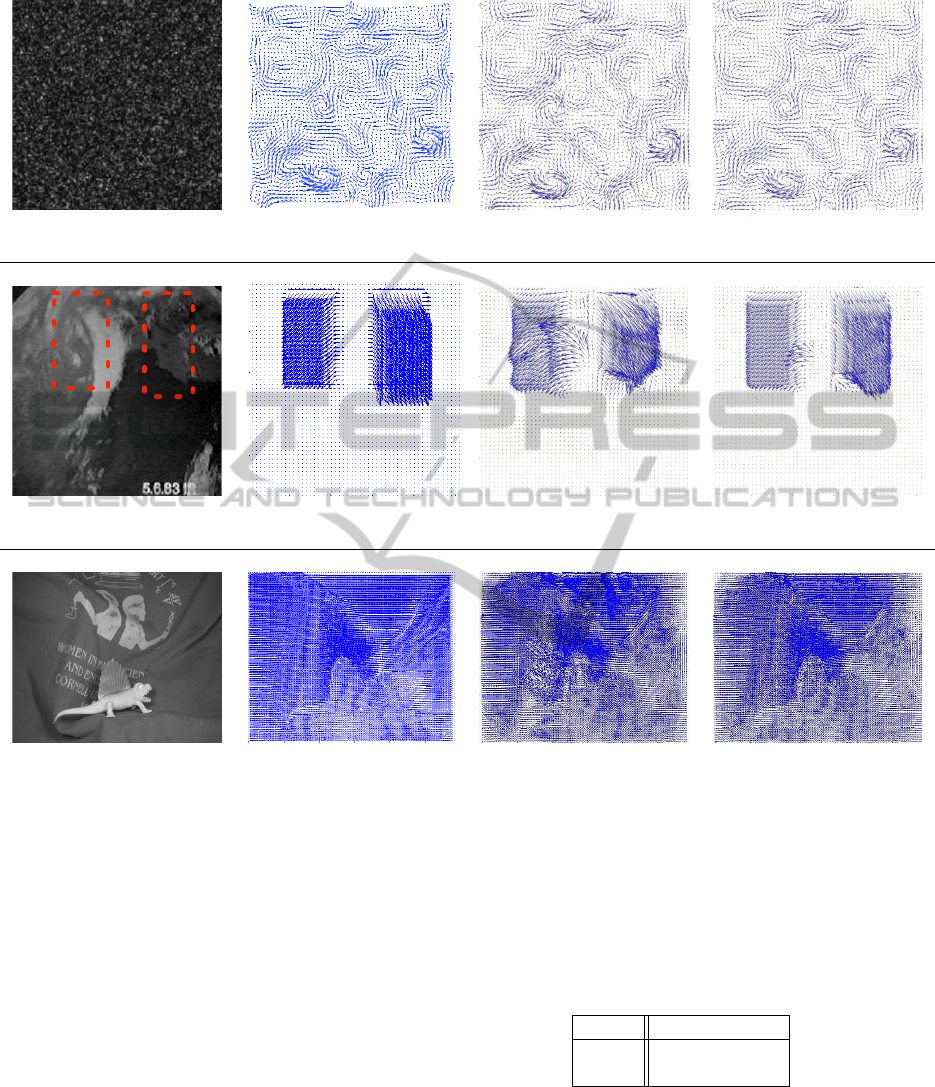
(a) (b) (c) (d)
(e) (f) (g) (h)
(i) (j) (k) (l)
Figure 3: Experiments on synthetic data. Top: synthetic DNS, Middle: synthetic general image made by hand; Bottom:
dimetrodon issued from the Middleburry database. For each pair, we respectively show one image of the sequence (a-e-i),
the synthetic velocity field (b-f-j); one estimation using the CONV technique (c-g-k) and one estimation using the proposed
AMR multi-resolution (d-h-l)
clearly affects the quality of the motion fields of fig-
ures 3(g–h). However from these two images, it ap-
pears clearly that the one issued from the AMR ap-
proach is better, as confirmed by the quantitative val-
ues of table 2. On this example, the first estimation
at the coarser level had some errors. There latter are
not corrected with a classical downscaling approach
whereas they are modified using our technique.
5.3 Synthetic Images of the
Middleburry Database
We have tested our approach on the “Dimetrodon”
pair of image issued from the Middleburry database.
The figure 3 embeds one image of the sequence (fig.
Table 2: Quantitative comparisons on the synthetic se-
quence with a Lucas-Kanade term embed in a multi-
resolution scheme with successive convolutions without any
assimilation (CONV) and the proposed multi-resolution us-
ing variational assimilation (AMR).
CONV AMR
AAE 9.02
o
5.62
o
RMSE 1.28 0.79
3(i)), the ground truth (fig. 3(j)), an estimated velocity
field with the CONV technique (fig. 3(k)) and with
the AMR one (fig. 3(l)). Associated numerical val-
ues are depicted in table 3. Here again, on this com-
plex motion with many discontinuities, the original
multi-resolution introduced in this paper outperforms
OPTIMAL CONTROL THEORY FOR MULTI-RESOLUTION PROBLEMS IN COMPUTER VISION - Application to
Optical-flow Estimation
141

Table 3: Quantitative comparisons on the dimetrodon
sequence with a Lucas-Kanade term embed in a multi-
resolution scheme with successive convolutions without any
assimilation (CONV) and the proposed multi-resolution us-
ing variational assimilation (AMR).
CONV AMR
AAE 7.95
o
6.50
o
RMSE 0.98 0.62
a usual one using similar observation terms. This is a
promising behavior.
5.4 Key Message
Various situations have been tested with these three
experiments: the first one exhibits a flow with many
interactions between scales, the second one is submit-
ted to the aperture problem whereas the third one is
composed of a more complex velocity field. From
the associated qualitative and quantitative values, it is
very interesting to point out that for a similar tech-
nique (i.e. the Lucas & Kanade estimaion), the new
multi-resolution approach is more competitive in all
applications. This is the key message of these experi-
ments.
6 CONCLUSIONS
In this paper, we have introduced an original mean
to perform multi-resolution strategies commonly used
in computer vision. These techniques, used to man-
age efficiently some simplifications (as linearization),
generally suffer from one drawback: their inability to
correct errors of coarser resolutions. Errors are indeed
most of the time propagated along the scales. In this
study, we have exploited a framework issued from op-
timal control theory and in particular variational data
assimilation to solve this issue. The general idea of
variationaldata assimilation techniques consist in per-
forming a set of forward/backward integrations of a
dynamical system to estimate a system state. Applied
to a scale-space equations, we have derived a consis-
tent mathematical framework to perform any multi-
resolution scheme in a set of forward/backward inte-
grations that in practice correspond to a set of down-
scaling/upscaling estimations.
We have validated the idea on a simple Lucas-
Kanade motion estimation technique for three syn-
thetic pair of images corresponding to various situ-
ations. The experimental results reveal that for all
tested images, our multi-resolution approach outper-
forms classic ones, which is a very interesting and
promising conclusion. As future works, we will
use more advanced observation terms associated with
non-linear scale space dynamics able to preserve dis-
continuities.
REFERENCES
Alvarez, L., Weickert, J., and S´anchez, J. (2000). Reli-
able estimation of dense optical flow fields with large
displacements. International Journal of Computer Vi-
sion, 39(1):41–56.
Baatz, M. and Schaape, A. (2000). Multiresolution Seg-
mentation: an optimization approach for high qual-
ity multi-scale image segmentation. In Strobl, J., ed-
itor, Angewandte Geographische Informationsverar-
beitung XII. Beitr¨age zum AGIT-Symposium Salzburg
2000, Karlsruhe, Herbert Wichmann Verlag, pages
12–23.
Bajcsy, R. and Kovacic, S. (1989). Multiresolution elas-
tic matching. Computer Vision, Graphics, and Image
Processing, 46(1):1 – 21.
Baker, S. and Matthews, I. (2004). Lucas-Kanade 20 Years
On: A Unifying Framework. International Journal of
Computer Vision, 56(3):221–255.
Baker, S., Scharstein, D., Lewis, J., Roth, S., Black, M.,
and Szeliski, R. (2007). A Database and Evaluation
Methodology for Optical Flow. In Int. Conf. on Comp.
Vis., ICCV 2007.
Baker, S., Scharstein, D., Lewis, J. P., Roth, S., Black, M. J.,
and Szeliski, R. (2010). A Database and Evaluation
Methodology for Optical Flow. International Journal
of Computer Vision, 92(1):1–31.
Barron, J., Fleet, D., Beauchemin, S., and Burkitt, T.
(1994). Performance Of Optical Flow Techniques. In-
ternational Journal of Computer Vision, 12(1):43–77.
Bennett, A. (1992). Inverse Methods in Physical Oceanog-
raphy. Cambridge University Press.
Brox, T., Bruhn, A., Papenberg, N., and Weickert, J. (2004).
High accuracy optical flow estimation based on a the-
ory for warping. pages 25–36. Springer.
Burt, P. (1988). Smart sensing within a pyramid vision ma-
chine. Proceedings of the IEEE, 76(8):1006 – 1015.
Corpetti, T., H´eas, P., M´emin, E., and Papadakis, N. (2009).
Pressure image assimilation for atmospheric motion
estimation. Tellus Series A: Dynamic Meteorology
and Oceanography, 61(1):160–178.
Corpetti, T. and M´emin, E. (2012). Stochastic uncer-
tainty models for the luminance consistency assump-
tion. IEEE Trans. on Image Processing, to appear.
Corpetti, T., M´emin, E., and P´erez, P. (2002). Dense Esti-
mation of Fluid Flows. IEEE Transactions on Pattern
Analysis and Machine Intelligence, 24(3):365–380.
Delanay, A. and Bresler, Y. (1998). Globally convergent
edge-preserving regularized reconstruction: an appli-
cation to limited-angle tomography. IEEE Trans. Im-
age Processing, 7(2):204–221.
Eck, M., DeRose, T., Duchamp, T., Hoppe, H., Lounsbery,
M., and Stuetzle, W. (1995). Multiresolution analy-
sis of arbitrary meshes. In Proceedings of the 22nd
VISAPP 2012 - International Conference on Computer Vision Theory and Applications
142

annual conference on Computer graphics and inter-
active techniques, SIGGRAPH ’95, pages 173–182,
New York, NY, USA. ACM.
Galvin, B., McCane, B., Novins, K., Mason, D., and Mills,
S. (1998). Recovering motion fields: an analysis of
eight optical flow algorithms. In Proc. British Mach.
Vis. Conf., Southampton.
Geman, D. and Reynolds, G. (1992). Constrained Restora-
tion and The Recovery Of Discontinuities. IEEE
Trans. Pattern Anal. Machine Intell., 14(3):367–383.
Horn, B. and Schunck, B. (1981). Determining optical flow.
Artificial Intelligence, 17(1-3):185–203.
Huber, P. (1981). Robust Statistics. John Wiley & Sons.
Le Dimet, F.-X. and Talagrand, O. (1986). Variational algo-
rithms for analysis and assimilation of meteorological
observations: theoretical aspects. Tellus, pages 97–
110.
Lions, J.-L. (1971). Optimal control of systems governed by
PDEs. Springer-Verlag.
Lucas, B. and Kanade, T. (1981). An iterative image regis-
tration technique with an application to stereo vision.
International joint conference on artificial, 130:121–
130.
Mallat, S. G. (1989). A theory for multiresolution signal de-
composition: the wavelet representation. IEEE Trans-
actions on Pattern Analysis and Machine Intelligence,
11:674–693.
Mitiche, A. and Bouthemy, P. (1996). Computation of im-
age motion: a synopsis of current problems and meth-
ods. Int. Journ. of Comp. Vis., 19(1):29–55.
Ojala, T., Pietikainen, M., and Maenpaa, T. (2002). Mul-
tiresolution gray-scale and rotation invariant texture
classification with local binary patterns. IEEE Trans-
actions on Pattern Analysis and Machine Intelligence,
24:971–987.
Talagrand, O. (1997). Assimilation of observations, an in-
troduction. J. Meteor. Soc. Jap., 75:191–209.
Talagrand, O. and Courtier, P. (1987). Variational assimi-
lation of meteorological observations with the adjoint
vorticity equation. {I}: Theory. J. of Roy. Meteo. soc.,
113:1311–1328.
Vidard, P., Blayo, E., Le Dimet, F.-X., and Piacentini, A.
(2000). 4D Variational Data Analysis with Imper-
fect Model. Flow, Turbulence and Combustion, 65(3-
4):489–504.
Yuan, J., Schnoerr, C., and M´emin, E. (2007). Discrete or-
thogonal decomposition and variational fluid flow es-
timation. Journ. of Mathematical Imaging and Vision,
28(1):67–80.
OPTIMAL CONTROL THEORY FOR MULTI-RESOLUTION PROBLEMS IN COMPUTER VISION - Application to
Optical-flow Estimation
143