MINIMALLY OVERLAPPING PATHS SETS FOR CLOSED
CONTOUR EXTRACTION
Julien Mille
1
, S
´
ebastien Bougleux
2
and Laurent Cohen
3
1
Universit
´
e de Lyon, CNRS, Universit
´
e Lyon 1, LIRIS, UMR5202, F-69622, Villeurbanne, France
2
Universit
´
e de Caen Basse-Normandie, CNRS, GREYC, UMR6072, F-14050, Caen, France
3
Universit
´
e Paris-Dauphine, CNRS, CEREMADE, UMR7534, F-75016, Paris, France
Keywords:
Segmentation, Boundary Extraction, Minimal Path, Active Contour, Overlap.
Abstract:
Active contours and minimal paths have been extensively studied theoretical tools for image segmentation. The
recent geodesically linked active contour model, which basically consists in a set of vertices connected by paths
of minimal cost, blend the benefits of both concepts. This makes up a closed piecewise-defined curve, over
which an edge or region energy functional can be formulated. As an important shortcoming, the geodesically
linked active contour model in its initial formulation does not guarantee to represent a simple curve, consistent
with respect to the purpose of segmentation. In this paper, we propose to extract a similarly piecewise-defined
curve from a set of possible paths, such that the resulting structure is guaranteed to represent a relevant closed
curve. Toward this goal, we introduce a global constraint penalizing excessive overlap between paths.
1 INTRODUCTION
Methods addressing the problem of two-phase seg-
mentation based on energy minimization techniques
and variational principles provide a solid mathemati-
cal background, and have proven to find suitable so-
lutions in many practical situations. Among them,
active contour models consist in deforming an ini-
tial curve until it captures the boundary of the tar-
get object. Whether they are implemented in an ex-
plicit fashion or using level sets, their evolution is usu-
ally driven by gradient descent of the Euler-Lagrange
equation, which makes them sensitive to local min-
ima, specifically in the presence of noisy images.
Consequently, the quality of the resulting segmenta-
tion strongly depends on the initial contour position.
Several attempts have been made to reduce this sen-
sitivity, including the addition of terms such as the
balloon force (Cohen, 1991) or the use of discrete op-
timization heuristics such as dynamic programming
(Amini et al., 1990) or greedy algorithms (Williams
and Shah, 1992). However, these methods still lead to
a local minimum of the energy.
To overcome sensitivity to local minima, (Co-
hen and Kimmel, 1997) proposed to find a global
minimum of the geodesic active contour functional,
provided that one or two points of the target object
boundary are initially supplied by the user. The result-
ing global geodesic curve, which can be respectively
closed or open, is efficiently derived from the solution
of the Eikonal equation obtained with the Fast March-
ing method (Tsitsiklis, 1995; Sethian, 1996). Since
the control points are fixed and must be located on the
target contour, this latter model does not represent a
curve which deforms its shape. Moreover, due to the
restricted number of these points, the geodesic may
fail to capture a relevant contour if the image is too
noisy, not enough contrasted, or if the target contour
is too lengthy. While several methods concentrate
on avoiding this second drawback (Benmansour and
Cohen, 2009) (Benmansour and Cohen, 2011) (Kaul
et al., 2010), the geodesically linked active contour
model of (Mille and Cohen, 2009) allows to overcome
the first one. This latter model combines the advan-
tages of geodesics with the ones of greedy algorithms
in order to deform a piecewise geodesic curve. More-
over, it is also able to include region-based energies,
such as the minimal variance term proposed by (Chan
and Vese, 2001), or even shape prior terms. Whereas
this model is relatively robust to local minima, it can
fail to construct a valid closed curve, from the initial-
ization step to the end of the evolution.
To overcome this drawback, we design a new en-
ergy functional allowing to find a piecewise smooth
curve with minimal overlapping. Given several pos-
sible relevant paths, subsequently referred to as ad-
259
Mille J., Bougleux S. and Cohen L..
MINIMALLY OVERLAPPING PATHS SETS FOR CLOSED CONTOUR EXTRACTION.
DOI: 10.5220/0003843102590268
In Proceedings of the International Conference on Computer Vision Theory and Applications (VISAPP-2012), pages 259-268
ISBN: 978-989-8565-03-7
Copyright
c
 2012 SCITEPRESS (Science and Technology Publications, Lda.)

missible paths, the key idea of our contribution is to
select the combination of paths generating the most
relevant contour. In this extent, we introduce an en-
ergy functional, combining contour and region terms
with a novel overlapping measure.The construction
of admissible paths, the overlapping energy as well
as the selection of the optimal combination of paths
are described in Section 3. The effectiveness of our
extended geodesically linked active contour model,
whether given initial points are located on the target
contour or far from it, is shown in Section 4 through
several experiments. The concepts on which relies the
proposed approach are recalled in the following sec-
tion.
2 RELATED CONCEPTS
2.1 Minimal Paths
To extract structures in a given image I : D → R
d
,
(Cohen and Kimmel, 1997) proposed to find curves
of minimal length according to an heterogeneous
isotropic metric defined from a potential P : D →R
∗+
.
This potential, which is chosen to take lower values
on the structure of interest, allows to measure the
length of piecewise smooth curves γ:[0, 1]→ D as fol-
lows:
L[γ] =
Z
1
0
P(γ(u))


γ
0
(u)


du. (1)
In the context of contour extraction, curves should be
located along edges. The potential is thus defined as
P=g +w, where g: D → R
+
is a decreasing function
of the gradient magnitude of the image (usually con-
volved with the derivatives of a Gaussian with given
standard deviation σ),
g(x) =
1
1 +
k
∇(K
σ
∗ I)(x)
k
(2)
and w∈R
∗+
is a regularizing constant. The target im-
age structure is then extracted by finding a path of
minimal length among all paths connecting two given
points x
1
and x
2
located on the structure
argmin
γ⊂D
{
L[γ]
}
s.t.

γ(0) = x
1
γ(1) = x
2
. (3)
Such a globally defined minimal path is called a
geodesic. The solution of minimization problem (3)
can be obtained by considering the geodesic distance
map, also referred to as the minimal action map,
U
v
:D →R
+
which assigns, to each point x ∈D, the
length of the minimal path connecting x to a given
point v∈D:
U
v
(x) = inf
γ
{
L[γ]
}
s.t.

γ(0) = v,
γ(1) = x.
(4)
This map is the unique viscosity solution of the
Eikonal equation

k
∇U
v
(x)
k
= P(x), ∀x ∈ D \{v},
U
v
(v) = 0,
(5)
see for instance (Crandall et al., 1992). This allows
to replace optimization problem (4) by a partial dif-
ferential equation. Its discrete version, on a cartesian
grid, can be efficiently solved by the Fast Marching
(FM) method in O(N log N) operations, where N is
the number of grid points (Tsitsiklis, 1995; Sethian,
1996; Sethian, 1999). Once the distance map has been
numerically computed, the minimal path between v
and any other point x of D can be extracted by a gra-
dient descent on U
v



γ
0
(u) = −
∇U
v
(γ(u))
k
∇U
v
(γ(u))
k
,
γ(0) = x,
(6)
that corresponds to a back-propagation starting from x
until v is reached. In practice, since the FM is a mono-
tonically front propagation method, finding the mini-
mal path bewteen two points does not require to com-
pute the distance on the whole domain D. Starting
from one point, the FM can be stopped when the sec-
ond point is reached, ensuring that the minimal path
can be extracted with (6).
The minimal path approach is not restricted to ex-
tract an open curve, provided its endpoints. In partic-
ular, in the context of object extraction, it is able to
find a closed curve, provided only one point on the
target object boundary. The closed curve is obtained
by detecting a saddle point of the distance map and
then by performing two back-propagations, in oppo-
site directions, starting from this saddle point (Cohen
and Kimmel, 1997). Whether the curve is closed or
open, the minimal path approach can fail to extract
the desired curve. As depicted in Fig. 1(d), some por-
tions of the minimal path do not follow the desired
curve. This happens for instance when P is too noisy
or not enough contrasted, when the length of the tar-
get curve is too important, or when the regularization
constant w is too high. This undesirable behaviour
hides a sampling problem, that is one or two points
are usually not enough to capture the whole desired
curve.
To overcome this drawback, several ap-
proaches aim at finding a piecewise geodesic
curve Γ =(V, {γ
i
}
i
), where V ={v
i
}
i
is a set of ver-
tices that samples the structure to extract, and {γ
i
}
i
is the set of geodesics connecting pairs of succesive
vertices (see Fig. 1(e)):
VISAPP 2012 - International Conference on Computer Vision Theory and Applications
260

(a) (b) (c) (d) (e)
Figure 1: (a) Input image. (b) Potential P. (c) Geodesic between two given points. (d) Undesirable sructure extraction. (e)
Piecewise geodesic curve.
γ
i
= argmin
γ
{
L[γ]
}
s.t.

γ(0) = v
i
,
γ(1) = v
i+1
.
(7)
Given an initial vertex set, new vertices can be re-
cursively and efficiently detected in several practical
situations such that the resulting piecewise geodesic
curve matches the desired structure. See (Benman-
sour and Cohen, 2009; Peyr
´
e et al., 2010) for a com-
plete survey. In Section 3 we propose an alternative
approach to overcome this drawback when a closed
curve needs to be extracted. This approach is closely
related to the geodesically linked active contour de-
scribed in the following section.
2.2 The Geodesically Linked Active
Contour Model
In order to extract an object from an image, (Mille and
Cohen, 2009) proposed an active contour model ex-
plicitely represented by a closed piecewise geodesic
curve, allowing initialization inside the object or
around the object boundary. The optimal contour
is defined as the piecewise geodesic closed curve
Γ=(V, {γ
i
}
1≤i≤n
) that minimizes a weighted sum of
edge-based and region-based energy functionals:
E[Γ] = ω
edge
E
edge
[Γ] + ω
region
E
region
[Γ]. (8)
The edge-based energy integrates the edge indicator
function g (Eq. (2)) along the geodesics
E
edge
(Γ) =
1
|Γ|
n
∑
i=1
Z
1
0
g(γ
i
(u))


γ
0
i
(u)


du. (9)
In order not to penalize lengthy contours, it is normal-
ized by the euclidean length
|Γ| =
n
∑
i=1
Z
1
0


γ
0
i
(u)


du.
One may note that the edge indicator g is used instead
of the potential P so that the euclidean component of
the curve length is not taken into account. This en-
sures that short curves, which could be undesirable
shortcuts, are not preferred over longer ones. This
edge term may be associated with a balloon term sim-
ilar to the one introduced in (Cohen, 1991) in order
to increase the capture range of the contour when lo-
cated far from the object boundary.
In addition, the region-based energy allows to
overcome limitations of the edge-based only model,
in particular when dealing with noisy, low-constrasted
or textured images. (Mille and Cohen, 2009) pro-
posed to use a modified version of the two-phase
piecewise constant segmentation model developped
by (Chan and Vese, 2001). Assuming that curve Γ
partitions the image into inner region Ω
in
and outer
region Ω
out
, the region term is expressed as the sum
of inner and outer image variances:
E
region
[Γ] =
1
|
Ω
in
|
Z
Ω
in
k
I(x) − µ
in
k
2
dx
+
1
|
Ω
out
|
Z
Ω
out
k
I(x) − µ
out
k
2
dx,
(10)
where µ
in
and µ
out
are average colors in these regions.
Following (Mille, 2009), a relaxed image homogene-
ity term focusing on the vicinity of the curve, referred
to as narrow band region term, was also addressed as
a possible replacement for the previous region term.
Evolution of active contours, whether they are im-
plemented explicitly or in a level-set fashion, is usu-
ally performed with gradient descent of the Euler-
Lagrange equation. However, in the present case,
the energy cannot be differentiated with respect to a
given vertex v
i
. It depends on geodesics linked to v
i
,
which are not expressed in closed form. Hence, the
piecewise geodesic structure is evolved thanks to a
greedy algorithm similar in principle to the one pro-
posed in (Williams and Shah, 1992), which is discrete
by nature and does not imply differentiation. Basi-
cally, vertices are moved in local windows in order to
minimize the selected energy. Let W
N
be a normal-
oriented window of length m centered at vertex v
i
:
W
N
(v
i
) =

v
i
+ kn
i



k = −
m
2
· ·
m
2

MINIMALLY OVERLAPPING PATHS SETS FOR CLOSED CONTOUR EXTRACTION
261

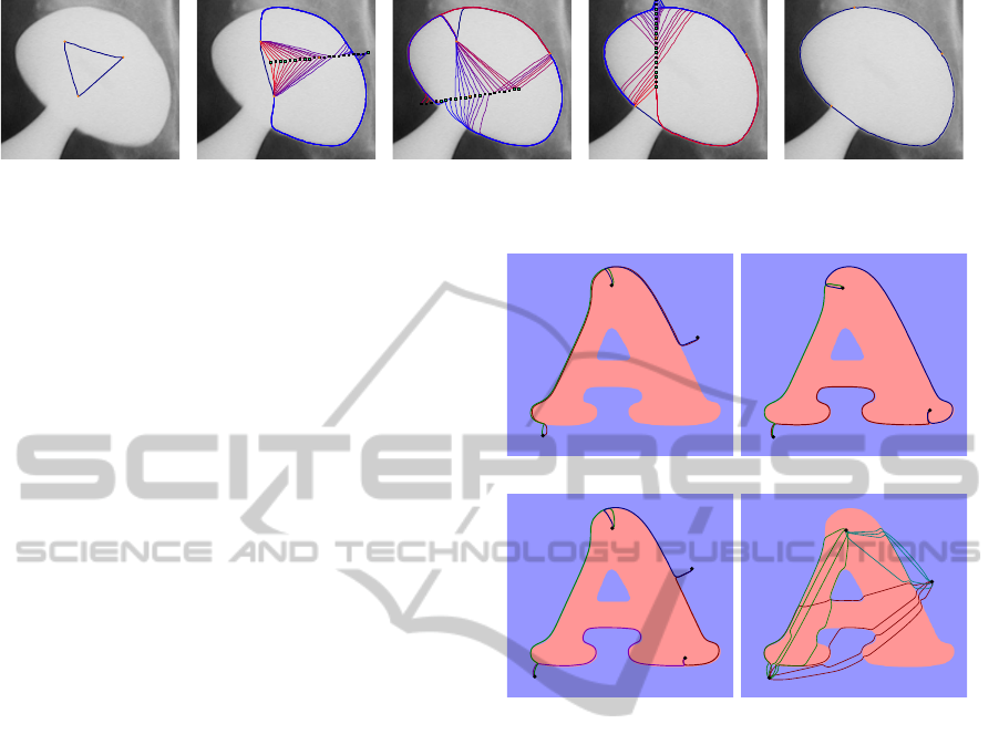
Figure 2: Evolution of geodesically linked active contour: in the evolution steps, all test geodesics from neighboring vertices
to test positions in windows are represented.
where n
i
is the inward unit normal vector, esti-
mated by finite difference on corresponding points on
geodesics γ
i
and γ
i+1
, respectively. Greedy evolution
is performed by moving vertex v
i
to the position in
the window which corresponding geodesically linked
contour has the smallest energy E. Let us consider a
test position
˜
v
i
belonging to the window, and its as-
sociated test geodesics
˜
γ
i−1
and
˜
γ
i
linking it to the
neighbors of v
i−1
and v
i+1
, respectively. The evolu-
tion scheme for vertex v
i
is formalized by the itera-
tion:
v
(t+1)
i
= argmin
˜
v
i
∈W
N

v
(t)
i

E(
˜
Γ)
where
˜
Γ is the tested piecewise geodesic curve:
˜
Γ = {γ
1
, ..., γ
i−2
,
˜
γ
i−1
,
˜
γ
i
, γ
i+1
, ..., γ
n
} (11)
The behavior of the geodesically linked active con-
tour is depicted in Fig. 2. We can observe that it is
able to capture accurately the object boundaries with
a reduced number of vertices.
While the geodesically linked active contour
model allows to blend the benefits of minimal paths
and region-based terms, it turns out to have a sig-
nificant drawback, as its initial state is not necessar-
ily a simple closed curve. As depicted in Fig. 3(a),
this can occur when the initial vertices are unevenly
distributed around the target boundary. In this case,
geodesics are very likely to gather on particular sides
of the target instead of roughly covering the boundary.
The reason is that each geodesic is generated indepen-
dently of the others, such that the obtained piecewise-
geodesic curve does not depend on the visiting order
of pairs of adjacent vertices. This undesirable phe-
nomenon may occur either as soon as the geodesically
linked contour is initialized, or after several evolution
steps on a previously well initialized contour.
As in Section 2.1, this problem can be seen as a
sampling one. Intuitively, one could think of impos-
ing evenly spaced vertices, as depicted in Fig. 3(b),
or adding vertices near the parts of the target bound-
ary which are not covered by the piecewise geodesic
curve, like in Fig. 3(c). In the considered context,
such sampling criteria are difficult to express, since
v
1
v
2
v
3
v
1
v
2
v
3
(a) (b)
v
1
v
2
v
3
v
4
v
1
v
2
v
3
(c) (d)
Figure 3: Towards a relevant initialization of the geodesi-
cally linked active contour model: (a) undesirable over-
lapping with unevenly spaced vertices, (b) improvement
by even spacing of vertices, (c) improvement by addition
of vertex, (d) admissible paths sets between pairs of ver-
tices with K = 4 paths per pair and high regularization con-
stant w.
the target boundary is unknown and applications usu-
ally need minimal user interaction. Otherwise, one
could think of imposing hard constraints on the over-
lapping between paths or penalizing paths enclosing
a region with excessively small area, but the indepen-
dent construction of paths prevents such constraints
to be implemented. We address this shortcoming in
what follows.
3 FINDING THE BEST PATH SET
To overcome the drawbacks of the geodesically linked
active contour model, we focus on determining a
more relevant contour representation which preserves
the advantages of piecewise geodesic curves. Assum-
ing that several possible relevant paths linking suc-
cessive vertices are available, the idea of our contri-
VISAPP 2012 - International Conference on Computer Vision Theory and Applications
262

bution is to select the combination of paths generat-
ing the most relevant boundary curve. This piecewise
smooth closed curve is built by selecting a single path
from each set, related to each pair of successive ver-
tices. The relevancy of the generated contour is mea-
sured by an energy functional, combining contour and
region terms with an overlapping measure. This last
term ensures the resulting curve to minimally overlap.
3.1 Sets of Admissible Paths
Let V = {v
i
}
1≤i≤n
be a sequence of n given vertices.
Instead of a single geodesic γ
i
for each pair of suc-
cessive vertices v
i
and v
i+1
, we consider a set S
i
of K
admissible paths available for this pair, as exemplified
in Fig. 3(d):
S
i
= {γ
i, j
}
1≤ j≤K
Paths in S
i
are sorted by cost in ascending order, so
that γ
i,1
actually corresponds to the minimal path be-
tween v
i
and v
i+1
whereas the remaining curves γ
i, j
,
2 ≤ j ≤ K, are only short paths of increasing cost.
Moreover, all paths in S
i
are constrained to be pair-
wise disjoint, except at their endpoints, which is for-
mulated as the following condition:
γ
i, j
1
(u) 6= γ
i, j
2
(v),
∀( j
1
, j
2
) ∈ [1..K]
2
, j
1
6= j
2
,
∀(u, v) ∈]0, 1[
2
, u 6= v.
One may notice that the current approach is more
constrained than the so-called K shortest paths prob-
lem (Yen, 1971; Eppstein, 1998), which, in its ba-
sic formulation, does not impose paths to be disjoint.
In the present case, the non-overlap constraint sim-
plifies the generation of several paths. Intuitively, in a
graph, the disjoint paths between a pair of vertices can
be found by running several instances of the shortest
path algorithm, after removal of vertices and incident
edges belonging to already found paths.
In our approach, recall that paths are extracted us-
ing the Fast Marching method. Hence, the K admis-
sible paths are built by successive deletion of already
existing paths from the potential map. Curve γ
i,1
is
the minimal path between v
i
and v
i+1
in the space
endowed by the initial potential P
1
= P. Once the
minimal path γ
i,1
has been computed, the second ad-
missible path γ
i,2
is sought under the constraint that
it should not pass through points belonging to γ
i,1
.
Hence, γ
i,2
is not a geodesic in the space induced by
potential P, but in the space induced by a modified
potential P
2
. The deletion of γ
i,1
in the modified po-
tential map is achieved by setting the potential to +∞
at all points of the geodesic. Extending this princi-
ple to the construction of the j
th
admissible path γ
i, j
as shown in Fig. 4, a recursive definition of potential
functions can be written as:
P
j
(x) =

+∞ if x ∈ γ
i, j−1
P
j−1
(x) otherwise.
This leads to the following recursive definition of the
set of admissible paths:
γ
i, j
= argmin
γ

Z
1
0
P
j
(γ(u))


γ
0
(u)


du

s.t. γ
i, j
(0) = v
i
and γ
i, j
(1) = v
i+1
.
From a practical point of view, one may note that the
gradient descent scheme used to built path is contin-
uous, which generates path points with real coordi-
nates, whereas the potential is implemented on a dis-
crete grid. Hence, in order to set P
j
(x) to +∞, we
actually set the 4 integer points surrounding x to +∞.
3.2 Paths Configuration of Minimal
Cost
The computation of an admissible closed contour con-
sists in selecting one path out of each set S
i
, such that
the contour resulting from the concatenation of se-
lected paths exhibit desirable properties in the image.
One of these properties is that the generated contour
should be simple, i.e. non-intersecting. In practice,
it is reasonable to allow some overlapping between
paths. A natural example arises when vertices are
located far from the target boundaries, which might
cause several admissible paths to have common sec-
tions before splitting up. Hence, the non-overlapping
condition should be reformulated as a soft constraint.
Towards this purpose, we first introduce the overlap
measure O between two curves:
O[C
1
, C
2
] = max

1
|
C
1
|
Z
1
0
ψ[C
1
(u), C
2
]


C
1
0


du,
1
|
C
2
|
Z
1
0
ψ[C
2
(u), C
1
]


C
2
0


du

.
(12)
It may be considered as the similarity counterpart of
the modified Hausdorff distance (Dubuisson and Jain,
1994), as the integrated quantity is a proximity mea-
sure instead of a distance. Penalty functional ψ mea-
sures the cost of the proximity of point x to curve C .
We chose a truncated linear decreasing function of the
euclidean distance between x and its nearest point lo-
cated on C :
ψ[x, C ] = max

0, 1 − α min
v∈[0,1]

k
x − C (v)
k

,
where weight α controls the decreasing slope, which
is related to the fuzziness of the overlap cost. Note
that O is symmetrical and O[C , C ] = 1.
MINIMALLY OVERLAPPING PATHS SETS FOR CLOSED CONTOUR EXTRACTION
263

Figure 4: Successive potential maps P
j
(top row) and corresponding admissible paths γ
·, j
(bottom row) given two endpoints.
The computation of an admissible closed contour
can be formulated as determining the sequence of la-
bels {x
1
, x
2
, . . . , x
n
} ∈ [1..K]
n
minimizing an energy
functional E, where label x
i
corresponds to the cho-
sen path in set S
i
:
min
{x
1
,x
2
,···,x
n
}∈[1..K]
n
E [Γ (γ
1,x
1
, γ
2,x
2
, ·· · , γ
n,x
n
)],
where Γ (γ
1,x
1
, γ
2,x
2
, ...., γ
n,x
n
) is the closed contour
built by concatenation of paths γ
i,x
i
. It is subse-
quently shortened to Γ for simplicity. Energy E is
the mathematical formulation of required properties
of Γ within the image, extending the energy func-
tional (8) involved in the geodesically linked active
contour model. It is designed to penalize contours ex-
hibiting strongly overlapping sections, poorly fitting
to image edges or enclosing regions with high color
disparity:
E[Γ] = E
overlap
[Γ] + ω
edge
E
edge
[Γ]
+ ω
region
E
region
[Γ].
(13)
Weights ω
edge
and ω
region
are user-defined parameters
controlling the relative significance of the edge and
region terms over the overlap term. This last one is
defined by applying the overlap measure defined in
equation (12) over all pairs of paths:
E
overlap
[Γ] =
n−1
∑
i=1
n
∑
j=i+1
O

γ
i,x
i
, γ
j,x
j

.
The edge energy integrates the edge indicator func-
tion g along paths normalized by their euclidean
length:
E
edge
[Γ] =
n
∑
i=1
1
|
γ
i,x
i
|
Z
1
0
g(γ
i,x
i
(u))


γ
i,x
i
0
(u)


du.
Unlike the previous edge term in Eq. (9), normaliza-
tion by euclidean length is performed on each path
before summation. This makes E
edge
a separable sum
of path-wise terms, which is an advantageous prop-
erty for optimization (this point is further discussed
in subsection 3.3). As the current curve to be opti-
mized is closed, we propose to use a region term, sim-
ilar to (10), which combines image color variances of
the two regions delimited by the curve, as proposed
by (Chan and Vese, 2001):
E
region
[Γ] =
λ
|
Ω
in
|
Z
Ω
in
k
I(x) − µ
in
k
2
dx
+
1 − λ
|
Ω
out
|
Z
Ω
out
k
I(x) − µ
out
k
2
dx,
(14)
where λ∈[0, 1] controls the blending of the two terms.
While the overlap and the edge energy functionals
constitute the building blocks of the proposed model,
the region term can be easily replaced in specific sit-
uations, e.g. with piecewise-smooth models (Lankton
and Tannenbaum, 2008; Brox and Cremers, 2009) or
texture features (Sagiv et al., 2006).
3.3 Optimization
The best sequence of labels {x
1
, x
2
, ..., x
n
} is deter-
mined using a brute force search among the K
n
pos-
sible configurations. Note that all energy terms are
fully or partially precomputed before testing these
configurations. Trivially, the edge term needs to
be computed only once for each path. Overlap co-
efficients O[·, ·] are pre-computed between all pairs
of path and stored in an upper triangular similarity
matrix, allowing straightforward computation of the
overlap term.
VISAPP 2012 - International Conference on Computer Vision Theory and Applications
264

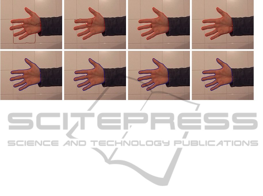
Figure 5: Robustness of contour extraction with respect to vertices locations: all admissible paths (top row) and selected
contour (bottom row).
Regarding the region term, Green’s theorem en-
ables to convert region integrals over Ω
in
(Γ) - and si-
multaneously over Ω
out
(Γ) = D\Ω
in
(Γ) - into a sum
of contour integrals over each path, according to the
following template formula. For any integrable func-
tion f over D, we have:
Z
Ω
in
(Γ)
f (x)dx =
n
∑
i=1
Z
1
0
F(γ
i,x
i
) · γ
i,x
i
0⊥
du (15)
where F is a vector field verifying div F = f . The
computation of color means and variances is therefore
separable over each path, which allows precomputa-
tion. Vector field F is obtained by integrating f along
the x and y-dimensions:
F(x, y) =

Z
x
0
f (t, y)dt ,
Z
y
0
f (x, t)dt

T
Two vector fields are computed once at every loca-
tion, for f = I and f =
k
I
k
2
, which allows color
means and variances, over inner and outer regions of
a given tested configuration Γ, to be efficiently deter-
mined.
4 EXPERIMENTS AND
DISCUSSION
We demonstrate the ability of the model to recover
closed boundaries of objects in natural color images,
given few user-provided points. These points are ei-
ther located on the target boundary, to assess the rele-
vancy of the proposed approach independently from
any deformation algorithm, or far from the bound-
ary, in order to show its benefits when integrated into
the deformation process of the geodesically linked ac-
tive contour model. In all experiments, regularization
weight w was set to 0.01, the RGB components being
assumed to vary from 0 to 1. Low values of w pre-
vent paths from creating undesirable shortcuts, there-
fore favouring high gradient edges. Reported execu-
tion times were obtained with a C++ implementation
running on a standard Intel Core2 Duo 2.8GHz archi-
tecture with 4Gb RAM.
4.1 From Points Localized on the
Contour
Fig. 5 depicts an experiment intended to demonstrate
the consistency of contour extraction with respect to
various initial locations of vertices. The closed con-
tour was generated given n = 2 vertices and K = 5
admissible paths. On the aforementioned architec-
ture, paths generation took 0.94s and contour selec-
tion took 0.14s. As neighboring areas are sufficiently
contrasted, the edge map alone turned out to be re-
liable enough, which allowed not to use the region
homogeneity term. Hence, only the overlap and edge
terms were used on this particular image. The pro-
posed approach proves to recover suitable contours
regardless of the positions of endpoints. In particu-
lar, vertices do not need to be evenly spaced along
the actual object boundary. One of the main bene-
fits of the proposed approach over classical minimal
path-based segmentation is the ability to formulate
a region-based criterion, as in classical active con-
tours. Figures 6 and 7 illustrate the interest of using
such criterion, as well as the overlap constraint. The
700×529 data in Fig. 6 was processed with n = 3 ver-
MINIMALLY OVERLAPPING PATHS SETS FOR CLOSED CONTOUR EXTRACTION
265

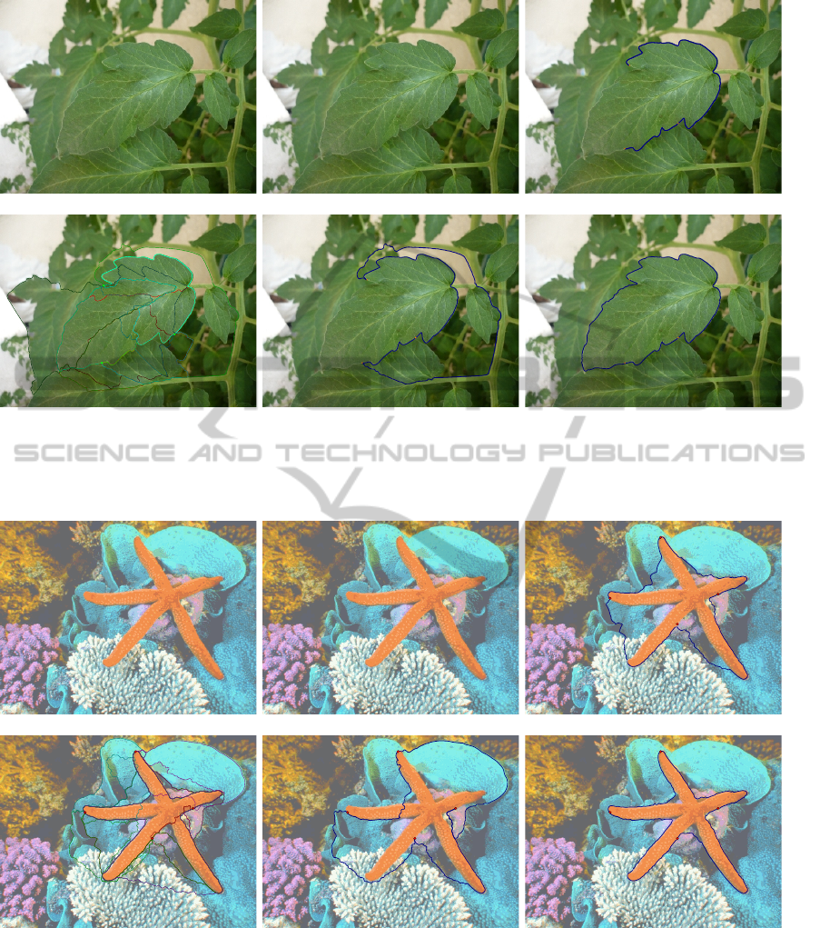
(a) (b) (c)
(d) (e) (f)
Figure 6: Influence of the region homogeneity term: (a) input image, (b) inverted gradient magnitude, (c) initial configuration
of the basic geodesically linked active contour (independent minimal paths), (d) all admissible paths, (e) selected contour with
overlap and edge terms, (f) selected contour with overlap, edge and region terms.
(a) (b) (c)
(d) (e) (f)
Figure 7: Influence of the region homogeneity term: (a) input image, (b) inverted gradient magnitude, (c) initial configuration
of the basic geodesically linked active contour (independent minimal paths), (d) all admissible paths, (e) selected contour with
overlap and edge terms, (f) selected contour with overlap, edge and region terms.
tices and K = 5 admissible paths per pair of succes-
sive vertices. Paths generation took 13.3s and con-
tour selection 3.9s. The annoying overlapping phe-
nomenon yielded by the basic geodesically linked ac-
tive contour is shown in Fig. 6(c). Incorporation of the
overlap constraint enables to generate a closed con-
tour, which remains nevertheless unrelevant with re-
spect to image partition. This can be explained by
VISAPP 2012 - International Conference on Computer Vision Theory and Applications
266

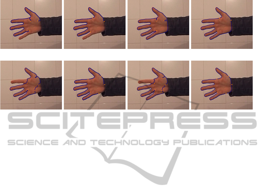
(a1) (a2) (b1) (b2)
(c1) (c2) (d1) (d2)
Figure 8: Integration of non-overlapping constraint in the geodesically linked active contour model. For each subfigure: (x1)
initial state, (x2) final state. (a & c) Basic geodesically linked active contour, (b & d) Geodesically linked active contour
model with non-overlapping constraint.
the fact that various edges, stronger that the actual
boundaries of the target object, can be encountered
in neighboring structures. This undesirable feature is
addressed by the addition of the region homogeneity
term (weight λ balancing the inner and outer region
terms was set to 1, as only the inner object is almost
homogeneous). The last experiment shown in Fig. 7
follows a similar principle, with n = 4 and K = 5,
on a 800 ×600 image. Reported execution times for
paths generation and contour selection are 22.5s and
7.8s, respectively. For this image, while the proposed
approach outperforms the geodesically linked active
contour model at its initialization, the resulting curve
fails to fully extract the desired contour, due to weak
edges near the object center. Since the object of inter-
est is textured, this could be improved by considering
a region energy that favors homogeneous textured re-
gions.
4.2 Integration into Deformation
Process
We report experiments where the proposed approach
was integrated into the evolution algorithm of the
geodesically linked active contour model, so that con-
tour extraction can be performed with initial points
located far from the target contour. The integra-
tion is as follows: during deformation, when displac-
ing a given vertex v
i
, tested geodesics
˜
γ
i−1
and
˜
γ
i
are built such that they do not overlap with existing
geodesics {γ
1
, ..., γ
i−2
, γ
i+1
, ..., γ
n
}. This is achieved
by deleting these existing geodesics in the potential
map, as described in subsection 3.1. The energy of
the tested contour is endowed with the overlap term
according to Eq. (13).
The proposed approach can solve the overlapping
problem arising in two different cases. The first case,
shown in Fig. 8(a), corresponds to an overlapping
present as soon as the contour is initialized and propa-
gated afterwards. On the other hand, the second case,
depicted in Fig. 8(c), shows the result of an overlap-
ping occuring during evolution of a well-initialized
curve. In both cases, the integration of our approach
when updating geodesics during evolution allows to
maintain a valid contour (Fig. 8(b) and Fig. 8(d)),
at the expense of additional time cost to check paths
configurations.
5 CONCLUSIONS AND
PERSPECTIVES
By searching the best paths configurations among sets
of admissible paths, given an energy functional com-
bining an edge fitting term, a region homogeneity
term and a novel overlap-penalizing energy, we aimed
at overcoming some important shortcomings arising
in geodesic-based segmentation. The introduced con-
straints allowed to guarantee consistent closed con-
tours, whether given initial points were located on the
target boundaries or far from them. Incorporation into
the geodesically linked active contour model demon-
strated the advantages of the approach.
MINIMALLY OVERLAPPING PATHS SETS FOR CLOSED CONTOUR EXTRACTION
267

Future work may focus on designing finer search
methods to determine the optimal set of paths, since
a basic brute force search was implemented so far. A
related possible investigation deals with the genera-
tion of admissible paths. In this extent, instead of
generating all admissible paths per pair of successive
vertices at initialization, one could think of an adap-
tive approach in which only necessary extra admissi-
ble paths would be created during the search process.
REFERENCES
Amini, A., Weymouth, T., and Jain, R. (1990). Using dy-
namic programming for solving variational problems
in vision. IEEE Transactions on Pattern Analysis and
Machine Intelligence, 12(9):855–867.
Benmansour, F. and Cohen, L. (2009). Fast object segmen-
tation by growing minimal paths from a single point
on 2D or 3D images. Journal of Mathematical Imag-
ing and Vision, 33(2):209–221.
Benmansour, F. and Cohen, L. (2011). Tubular struc-
ture segmentation based on minimal path method and
anisotropic enhancement. International Journal of
Computer Vision, 92(2):192–210.
Brox, T. and Cremers, D. (2009). On local region models
and a statistical interpretation of the piecewise smooth
Mumford-Shah functional. International Journal of
Computer Vision, 84(2):184–193.
Chan, T. and Vese, L. (2001). Active contours with-
out edges. IEEE Transactions on Image Processing,
10(2):266–277.
Cohen, L. (1991). On active contour models and balloons.
Computer Vision, Graphics, and Image Processing:
Image Understanding, 53(2):211–218.
Cohen, L. and Kimmel, R. (1997). Global minimum for
active contour models: a minimal path approach. In-
ternational Journal of Computer Vision, 24(1):57–78.
Crandall, M., Ishii, H., and Lions, P.-L. (1992). User’s guide
to viscosity solutions of second order partial differen-
tial equations. Bull. Amer. Math. Soc., 27:1–67.
Dubuisson, M.-P. and Jain, A. (1994). A modified Haus-
dorff distance for object matching. In 12
th
Inter-
national Conference on Pattern Recognition (ICPR),
pages 566–568, Jerusalem, Israel.
Eppstein, D. (1998). Finding the k shortest paths. SIAM
Journal of Computing, 28(2):652–673.
Kaul, V., Tsai, Y., and Yezzi, A. (2010). Detection of
curves with unknown endpoints using minimal path
techniques. In British Machine Vision Conference
(BMVC), pages 1–12, Aberystwyth, UK.
Lankton, S. and Tannenbaum, A. (2008). Localizing region-
based active contours. IEEE Transactions on Image
Processing, 17(11):2029–2039.
Mille, J. (2009). Narrow band region-based active contours
and surfaces for 2D and 3D segmentation. Computer
Vision and Image Understanding, 113(9):946–965.
Mille, J. and Cohen, L. (2009). Geodesically linked active
contours: evolution strategy based on minimal paths.
In 2
nd
International Conference on Scale Space and
Variational Methods in Computer Vision (SSVM), vol-
ume 5567 of LNCS, pages 163–174, Voss, Norway.
Springer.
Peyr
´
e, G., Pechaud, M., Keriven, R., and Cohen, L. (2010).
Geodesic methods in computer vision and graphics.
Foundations and Trends in Computer Graphics and
Vision, 5(3-4):197–397.
Sagiv, C., Sochen, N., and Zeevi, Y. (2006). Integrated ac-
tive contours for texture segmentation. IEEE Transac-
tions on Image Processing, 15(6):1633–1646.
Sethian, J. (1996). A fast marching level set method for
monotonically advancing fronts. Proceedings of the
National Academy of Science, 93(4):1591–1595.
Sethian, J. (1999). Level Sets Methods and Fast Marching
Methods. Cambridge University Press, 2nd edition.
Tsitsiklis, J. (1995). Efficient algorithms for globally op-
timal trajectories. IEEE Transactions on Automatic
Control, 40(9):1528–1538.
Williams, D. and Shah, M. (1992). A fast algorithm for
active contours and curvature estimation. Computer
Vision, Graphics, and Image Processing: Image Un-
derstanding, 55(1):14–26.
Yen, J. (1971). Finding the K shortest loopless paths in a
network. Management Science, 17(11):712–716.
VISAPP 2012 - International Conference on Computer Vision Theory and Applications
268