INTERACTIVE VISUAL ANALYSIS OF INTENSIVE

CARE UNIT DATA

Relationship between Serum Sodium Concentration, its Rate of Change

and Survival Outcome

Kre

simir Matkovi

, Heng Gan

, Andreas Ammer

, David Bennett

Werner Purgathofer

and Marius Terblanche

VRVis Research Center in Vienna, Vienna, Austria

Guy’s & St Thomas’ NHS Foundation Trust, London, U.K.

King’s College London and Guy’s & St. Thomas’ NHS Foundation Trust, London, U.K.

Keywords:

Interactive Visual Analysis, Coordinated Multiple Views, Intensive Care Unit Data.

Abstract:

In this paper we present a case study of interactive visual analysis and exploration of a large ICU data set. The

data consists of patients’ records containing scalar data representing various patients’ parameters (e.g. gender,

age, weight), and time series data describing logged parameters over time (e.g. heart rate, blood pressure).

Due to the size and complexity of the data, coupled with limited time and resources, such ICU data is often not

utilized to its full potential, although its analysis could contribute to a better understanding of physiological,

pathological and therapeutic processes, and consequently lead to an improvement of medical care. During the

exploration of this data we identiﬁed several analysis tasks and adapted and improved a coordinated multiple

views system accordingly. Besides a curve view which also supports time series with gaps, we introduced a

summary view which allows an easy comparison of subsets of the data and a box plot view in a coordinated

multiple views setup. Furthermore, we introduced an inverse brush, a secondary brush which automatically

selects non-brushed items, and updates itself accordingly when the original brush is modiﬁed. The case

study describes how we used the system to analyze data from 1447 patients from the ICU at Guy’s & St.

Thomas’ NHS Foundation Trust in London. We were interested in the relationship between serum sodium

concentration, its rate of change and their effect on ICU mortality rates. The interactive visual analysis led us

to ﬁndings which were fascinating for medical experts, and which would be very difﬁcult to discover using

conventional analysis methods usually applied in the medical ﬁeld. The overall feedback from domain experts

(coauthors of the paper) is very positive.

1 INTRODUCTION

The monitoring and management of patients in mod-

ern Intensive Care Units (ICU) is technology-driven

and use numerous high technology equipment. Each

of those has the ability to log various parameters.

Many physiological measurements (such as blood

pressure, body temperature, or heart rate, for exam-

ple), laboratory results, and treatment interventions

are routinely recorded. These measurements help in-

tensive care physicians to understand physiological,

pathological and therapeutic processes, and conse-

quently to improve medical care.

The data collected routinely in a modern ICU cre-

ates very large datasets containing in-depth time-var-

variant and time-invariant data. For various reasons

these datasets are generally not used to their full po-

tential. First, data is often stored on different propri-

etary systems each using difference storing and output

formats. Second, statistical models (particularly for

multi-level longitudinal data) are difﬁcult to develop

and require large datasets to improve estimate preci-

sion. Third, most clinical researchers do not possess

the statistical skills to develop complex models, while

statisticians generally lack the contextual understand-

ing of the biological and clinical processes needed to

develop the conceptual constructs for testing.

The use of data visualization techniques to gain

insight into large ICU datasets is a novel concept.

Historically, standard single and multi variable re-

648

Matkovi

c K., Gan H., Ammer A., Bennett D., Purgathofer W. and Terblanche M..

INTERACTIVE VISUAL ANALYSIS OF INTENSIVE CARE UNIT DATA - Relationship between Serum Sodium Concentration, its Rate of Change and

Survival Outcome.

DOI: 10.5220/0003844506480659

In Proceedings of the International Conference on Computer Graphics Theory and Applications (IVAPP-2012), pages 648-659

ISBN: 978-989-8565-02-0

 2012 SCITEPRESS (Science and Technology Publications, Lda.)

gression techniques are used to investigate associa-

tions between one or more predictor variables and an

outcome. The APACHE II (”Acute Physiology and

Chronic Health Evaluation II”) scoring system, for

example, is a severity of disease classiﬁcation sys-

tem, which was introduced in 1985 (Knaus et al.,

1985), and modiﬁed in 1991 (Knaus et al., 1991). The

APACHE II score is computed based on several mea-

surements after a patient enters an ICU, and indicates

how severe a disease is and the risk of death of the

patient. There are other scoring systems as well.

While sophisticated, the conventional techniques

require a high degree of training and do not provide

intuitive insights in the within-data relationships and

linkages. Here we test the ability of interactive visual

analysis to analyze a large ICU data set. Our goal is to

test if such a method is suitable for medical data ex-

ploration. We wanted to see if some new, hidden, cor-

relation can be found in the data which is not present

in standard scores. Although it seems straightforward,

such an analysis is far from trivial.

Data for 1447 patients was collected in the ICU at

Guy’s & St. Thomas’ NHS Foundation Trust, Lon-

don, UK. The ICU is completely paperless and all

medical data, including medical notes and prescrip-

tion charts, are stored centrally. On admission and

during the patient’s stay all parameters are logged and

the data is stored in a central database. The data set

is broadly divided into time-invariant (e.g. ID, age,

gender, admission diagnosis, survival, etc.) and time-

variant data (e.g. sodium concentration, blood pres-

sure, etc.). As we have scalar data and time series data

for every patient we used a data model introduced by

Konyha et al. (Konyha et al., 2006). Instead of hav-

ing only scalar values as attributes in patients records

this model supports time series as attributes. All time

series of one kind (e.g. blood pressure values as a

function of time) for all patients represent a family of

curves.

In this paper we describe how we examined the

association between serum sodium concentration, its

rate of change, and survival outcome. The paper is

written together with domain experts. We use a pow-

erful data preprocessing and a coordinated multiple

views (CMV) system to explore and analyze the data

by means of interactive visual analysis. In order to be

able to perform the study we have improved the curve

view (Konyha et al., 2006) to support different curve

lengths, and to depict gaps in time series. We also in-

tegrated a new summary view along with a box plot

view into the system and introduced a new interac-

tion – the inverse brush. Finally, we have modiﬁed an

existing CMV system in order to suit domain experts

needs. All improvements were made after numerous

common sessions with the domain experts. Unex-

pected ﬁndings and a very positive feedback from the

domain experts indicated that our approach is feasi-

ble, and demonstrated how interactive visual analysis

can increase understanding of ICU data and poten-

tially contribute to better medical care. The approach

has been preliminary introduced to the medical com-

munity by a poster at a major intensive care medicine

congress (Gan et al., 2011).

2 RELATED WORK

Using coordinated multiple views (CMV) is a com-

mon practice in interactive visual analysis. An

overview of CMV is provided by Roberts (Roberts,

2007). The task of visualizing time-oriented data

however needs additional consideration, reﬂected

by Shneiderman’s ”Task by Data Type Taxon-

omy” (Shneiderman, 2002), where temporal data is

identiﬁed as one of seven basic data types. Aigner et

al. (Aigner et al., 2007b; Aigner et al., 2007a) give

a good overview of characteristics of time-oriented

data and different methods of visualizing it accord-

ingly. According to Aigner et al. (Aigner et al.,

2007b) the time-oriented data in our case can be cate-

gorized as multivariate abstract data at time-points in

linear time shown in a static 2D representation. An

example of interactive visualization and exploration

of time-dependent data is the TimeSearcher appli-

cation by Hochheiser and Shneiderman. (Hochheiser

and Shneiderman, 2002; Hochheiser and Shneider-

man, 2004), who also developed visual query mecha-

nisms for ﬁnding patterns in time series data. Visual

queries allow the user to directly compose queries in

the visualization without the need of dealing with ad-

ditional sliders or input ﬁelds.

Additionally our time series data contains miss-

ing values, which requires extra consideration. Time

series data which is sampled regularly but contains

missing values can be seen as unregular sampled, or

event-based data. Aris et al. (Aris et al., 2005) devel-

oped for the TimeSearcher application four methods

to deal with such unevenly spaced time series data;

namely: sampled events, aggregated sampled events,

event index and interleaved event index. Since nei-

ther method meets all the requirements of our case –

the ﬁrst two methods introduce new data at the sam-

ple points, the latter two only consider the order of

events, not the speciﬁc time they appeared – we use a

different method in handling missing values.

There exist several approaches to visualize the

time-oriented data of a single patient record. Powsner

and Tufte (Powsner and Tufte, 1994) visualize time-

INTERACTIVE VISUAL ANALYSIS OF INTENSIVE CARE UNIT DATA - Relationship between Serum Sodium

Concentration, its Rate of Change and Survival Outcome

649

oriented data in small repeated graphs. LifeLines by

Plaisant et al. (Plaisant et al., 1996; Plaisant et al.,

1998) uses timelines with colored horizontal bars and

markers to indicate the point in time and the dura-

tion of actions or events (e.g. diagnosed symptoms

or treatments). However LifeLines lacks the ability

to visualize continuous data (e.g. fever curves). Bade

et al. (Bade et al., 2004) try to overcome this short-

coming by introducing height-coded timelines where

the height of the horizontal bar is depending of the

data of an associated time series. The approaches

mentioned in this paragraph seek to visualize many

or even all parameters and time series of one single

patient record as well as possible; we however are in-

terested in comparing parameters and time series of

multiple patient records and ﬁnding some relations

between them.

Multiple patient records were analyzed by Gresh

et al. (Gresh et al., 2002), who use information visual-

ization techniques to examine a large collection of pa-

tient records of bone marrow transplants at Hadassah

Hospital in Jerusalem, Israel. Gresh et al. generated

survivability curves for patients with mis-matched

transplant and fully matched transplant and compared

these for transplants received in the last ﬁve years

and prior to that. Surprisingly they initially found a

lower survival for the recent transplant patients, but in

subsequent discussions with the physicians they were

able to learn two of the reasons for that. First, the

hospital tends to be better at documenting death dates

than follow-up visits of surviving patients and second

the hospital specialized in the latter years in treating

more serious and complex cases. Although the sur-

vivability curves make use of time, there were no con-

tinuous time data in the dataset they investigated.

The mentioned before LifeLines were also used to

analyze multiple patient records by Wang et al. (Wang

et al., 2008) and Plaisant et al. (Plaisant et al., 2008).

They use aligning by sentinel events (e.g. the ﬁrst oc-

currence of a symptom) to discover patterns in elec-

tronic health records. Again they are not considering

continuous time data.

Finally Trobec at al. (Trobec et al., 2008) used a

CMV tool and a complex data model to analyze dif-

ferent statistical characteristics and time series from

ECG and respiration measurements from patients af-

ter heart transplantation. They used interactive visual

analysis and other, more conventional approaches.

3 ICU DATA

The dataset that we used in our analysis was created

using a commercial clinical information system (CIS;

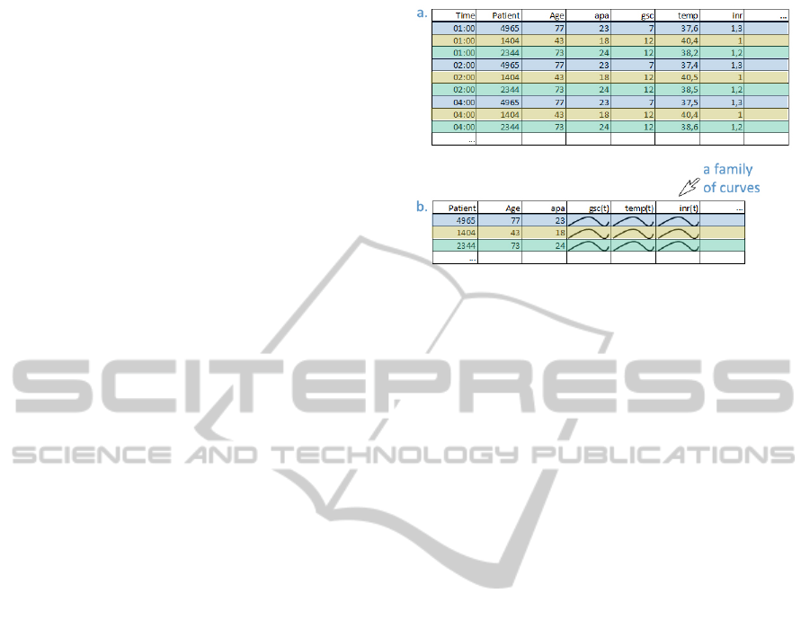
Figure 1: a. A conventional way of storing data. Each log

is a unique record containing patients data, time, and logged

parameters. b. A more complex data model allowing fami-

lies of curves. All records that belong to the same patients

form a single record. There is no time dimension, but in-

stead it is implicitly stored in a curve dimension. There is

gsc(t) now, e.g., in contrast to Time and gsc in the previous

case. We call all curves that belong to the same attribute a

family of curves.

CareVue, Phillips, The Netherlands) and contains one

record for each log. A record here contains patient

data and logged values together with logging time.

Figure 1a. shows such a case. In a simple data struc-

ture we would have a large table with as many rows as

there are records in the database, but since all records

of one patient belong together – they form a logical

unit – we group them to one record. Now a single

attribute is a time series and the number of rows is

equal to the number of patients. In this way we will

be able to follow data belonging to the same patient

more intuitively. Such a data organization reduces the

data size, but increases the data complexity (see Fig-

ure 1b.). At the same time it offers new possibilities

for analysis. The curves that emerged can be analyzed

using some advanced techniques which would be al-

most impossible (or very complicated) using conven-

tional queries and conventional data organization.

During the merging of the data, we noticed that

there are missing values in the time series, and that

time series are of different length. Some data (e.g.

physiological variables) are logged manually at least

hourly, while other data (e.g. laboratory results) are

logged via direct links with the institution’s computer

system. For various reasons missing data is com-

mon in clinical information systems (CIS). Reasons

include clinical need (e.g. a certain test is not clini-

cally indicate for a period of time), practical consid-

erations (e.g. a patient is temporarily transferred out

of the ICU for investigations), technical failure (e.g.

communication issues between the CIS and the insti-

tution’s computer network), or infrequently for main-

IVAPP 2012 - International Conference on Information Visualization Theory and Applications

650

Table 1: A subset of ICU data attributes.

Parameter Acronym Type

Age age numeric

ICU mortality idead numeric

APACHE II score apa numeric

Length of stay in ICU ilos numeric

Baseline venous oxy-

gen saturation

base

so2 numeric

Baseline plasma lactate

concentration

base lact numeric

Heart rate hr tsh time series

Mean arterial pressure map tsh time series

Plasma lactate concen-

tration

lact tsh time series

Venous oxygen satura-

tion

so2 tsh time series

Plasma sodium concen-

tration

na tsh time series

Plasma chloride con-

centration

cl tsh time series

C-reactive protein con-

centration

crp tsd time series

tenance/upgrades of the CIS itself. All time series

data start at the moment the patient enters the ICU,

and last for the time the patient is at the ICU, which

is different for each patient. As a consequence the

lengths of the time series in the dataset are different

for various patients. In order to cope with this issues

we have improved the curve view to support different

length time series.

During the data preprocessing step we have also

computed derived data needed in analysis. For the

time series data we have computed and stored: 1) the

number of small and large gaps; 2) the X and Y span

of time series; 3) the ﬁrst derivative – in order to ex-

plore the rise or fall in the family of curves, and 4) ba-

sic scalar aggregates such as minimum or maximum

of original and of derived families of curves. Some of

those derived values are scalar values, which means

that a curve from a family is described using a scalar

(one curve is represented by one number) and some of

them are time series aggregates (the ﬁrst derivative,

e.g.) where time series is represented with another

time series and a new family of curves is introduced.

We have even computed some scalar aggregates of de-

rived time series (maximum of the ﬁrst derivation, for

example).

We have more than 40 attributes in the data set

(numeric and time dependent), and we have computed

about 20 aggregates in total. Table 1 lists the most

relevant subset used in the examples described in the

paper.

4 INTERACTIVE VISUAL

ANALYSIS OF ICU DATA

In our analysis we use a coordinated multiple views

system which supports iterative multiple brushes. The

main idea of coordinated multiple views is to use

more views to depict various data dimensions. User

can interactively brush (select) a subset of data in one

view and all corresponding items in all other, linked,

views are highlighted. Remember our records are pa-

tients based, so when some items are highlighted in

one view the items belonging to the same patients are

highlighted in all other views. The tool supports com-

posite iterative brushing, i.e. it is possible to combine

more brushes using basic logical operations, and the

last brush is always combined with the previous se-

lection. Such a system allows for a quick information

drill down, and it is especially suitable for data explo-

ration and analysis of hidden correlations. After just a

few sessions with our medical experts we realized that

we needed a quite ﬁx view organization. We have di-

vided the main frame into four parts (Figure 2). We

have a data manipulation part on the left (”A” in the

Figure 2), exploration part (”B”) in the middle, sum-

mary part (”C”) on the right, and details on demand

part (”D”) in the lower part of the screen. The data

manipulation part shows all the dimensions with their

ranges and allows the user to easily ﬁlter out records

with unwanted values during the analysis. The explo-

ration part is the core part. It is often reconﬁgured

during the analysis. We will show excerpts from the

exploration part with a detailed description in the rest

of the paper. We mostly used four to six views in

this part, and if some tasks needed more views they

were depicted in additional ﬂoating views. The ﬂoat-

ing views contain only exploration views and are usu-

ally shown on a second monitor. The summary part

shows some statistical moments of the most important

dimensions in a boxplot along with a quick overview

of the different brushes. By simple triangular glyphs

depicting the differences between the selected sub-

sets and the overall dataset, relations between subsets

and dimensions can easily be noticed. Finally, experts

need details at the end of the drill down process. All

the available data for selected patients is shown and

can be exported if needed in the details on demand

part.

The data described in the previous sections has

some characteristics that required improvements of

the existing visualization system. We improved the

curve view as proposed by Konyha et al. (Konyha

et al., 2006) and we have introduced a summary view

along with a box plot view in a coordinated multiple

views setup. During our analysis sessions the medi-

INTERACTIVE VISUAL ANALYSIS OF INTENSIVE CARE UNIT DATA - Relationship between Serum Sodium

Concentration, its Rate of Change and Survival Outcome

651

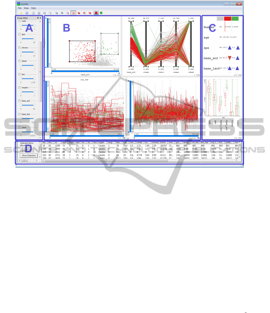
Figure 2: The coordinated multiple views system used. The views organization is ﬁx and deﬁned together with domain

experts. A. Data part shows all dimensions and their ranges. User can easily ﬁlter out records here. B. Exploration part used

for the interactive analysis. Views are freely conﬁgurable. There can be more views, and additional views can also be depicted

in a ﬂoating view. C. Summary part shows summary of selected dimensions. There are two views, summary overview and

box plot views. In case of multiple composite brushes a summary for each brush is shown. D. Details on demand – complete

data for each patient – are shown after drill down.

cal members of the team needed an ”inverse brush”.

In standard systems brushed items are usually shown

in contrast to a context, i.e. all items, but we wanted

to see the brushed items in context of all, along with

the non-brushed items in context of all, and the non-

brushed items in comparison to the brushed items. We

will describe each of our improvements to the CMV

system in the next subsections in more detail.

4.1 Depicting Gaps using a Curve View

The curve view as proposed by Konyha et al. (Konyha

et al., 2006) depicts all curves of a family simultane-

ously. In order to show the density of curves in a cer-

tain area a density based transparency is used. The

curves in our dataset have gaps, and the gaps cannot

be simply ignored. If gap start and end points would

be simply connected, values which might be wrong

are introduced without any warning. The user has to

know if data had been measured or if it is just miss-

ing. We propose to distinguish between small gaps

and large gaps (user can deﬁne the limits), and we de-

pict start and end points of all gaps using points (with

user deﬁned colors and sizes, different for large and

small gaps, and start and end points). Furthermore we

let the user choose the line type which will be used

to ”bridge” the gap if the user decides to draw a line

in a gap at all. If lines are not drawn the notion of

which curve segments belong together might be lost

in the case of many gaps. A mouse over function-

ality solves this problem. The whole curve is high-

lighted when the mouse is pointing to any of the gap

points. Figure 3a. illustrates the new curve view with

small gap points depicted in green, large gap points

depicted in red, and a yellow curve highlighted us-

ing the mouse over functionality. The crp tsd pa-

rameter is depicted in this ﬁgure. Although the ﬁgure

might seem crowded and not informative, in a linked

view setup the user can quickly drill down and reduce

the curves to a subset in focus. Figure 3b. and c.

show such subsets of curves in focus (red) and all

curves in context (gray). The curves of interest can

be seen clearly now. Proposed improvements helped

us in cleaning the data and in understanding what is

IVAPP 2012 - International Conference on Information Visualization Theory and Applications

652

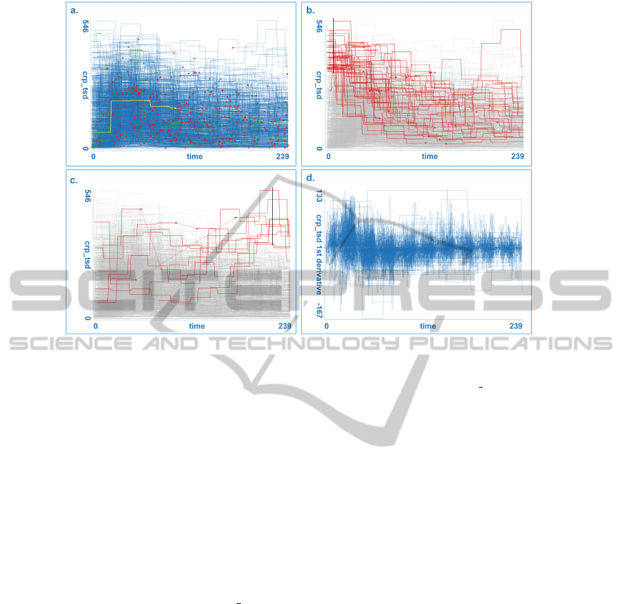
Figure 3: a. Enhanced curve view which shows all curves from a family simultaneously, with gap starting and ending points.

The yellow curve has been selected by simple mouse-over functionality. b. User selects all curves with high values at the

beginning (black line used for selection). Note that most of those curve sink with time, the crp tsd values become lower.

c. Curves with high values after 23 hours. Note one curve with a very long gap; values depicted using dashed line are most

probably wrong. d. Depicting the ﬁrst derivation aggregate will be very useful in the analysis later. Straight horizontal lines

indicate gaps, and represent an alternative way to see them.

missing. We assumed there were some gaps when we

started the analysis, but the number of gaps showed to

be higher then expected by medical experts and intro-

duced improvements were very welcomed, especially

during the data preparation phase.

As stated in section 3 we have used various ag-

gregated dimensions in the analysis. The ﬁrst deriva-

tion, primarily used to explore the rise and fall of cer-

tain parameters can be used to identify gaps as well.

Figure 3d. shows the ﬁrst derivative of cr p tsd (pa-

rameter showed in Figure 3a. - c.). Note the straight

line segments which correspond to gaps. Such a vi-

sualization of gaps (which is not a primary use of the

ﬁrst derivative aggregate) might be more useful some-

times.

4.2 Box Plot in the CMV

The medical experts in our team are used to the box

plot visualization. The box plot is a common and

convenient way to depict summaries of data (Tukey,

1977; McGill et al., 1978). In a multidimensional

data case, one box plot depicts summaries of one di-

mension (of course this is only possible for scalar di-

mensions). We have integrated a box plot view in the

CMV system. The view shows many adjacent box

plots. A relative scale (all box plots have the same

height) and an absolute scale is supported. Interest-

ingly, we used relative scale more often, as it was

clear to the experts that the overall ranges are not the

same. The box plot view is linked with all other views

and if something is brushed the box plot shows data

for context and for brushed data. Figure 4a. shows

a box plot view. Figure 4b. shows the same view in

a case where brushing is active. The box plots for

the brushed items are depicted in color (focus) and

are drawn on top of the gray box plots representing

all values (context). The user can easily compare the

values of the selection and the context. The focus is

a result of complex brushing in several other views.

User can combine brushes using boolean algebra, and

the box plot shows the distribution of the ﬁnal brush.

4.3 The Brush Overview View

The brush overview allows a quick comparison be-

tween the different selected subsets and the overall

data (see Figure 5). In a table layout where each col-

umn corresponds to a brush (i.e. a subset of the data)

and each row corresponds to a dimension, glyphs

and numerical values are depicted. The ﬁrst column

hereby corresponds to the overall dataset. The ﬁrst

INTERACTIVE VISUAL ANALYSIS OF INTENSIVE CARE UNIT DATA - Relationship between Serum Sodium

Concentration, its Rate of Change and Survival Outcome

653

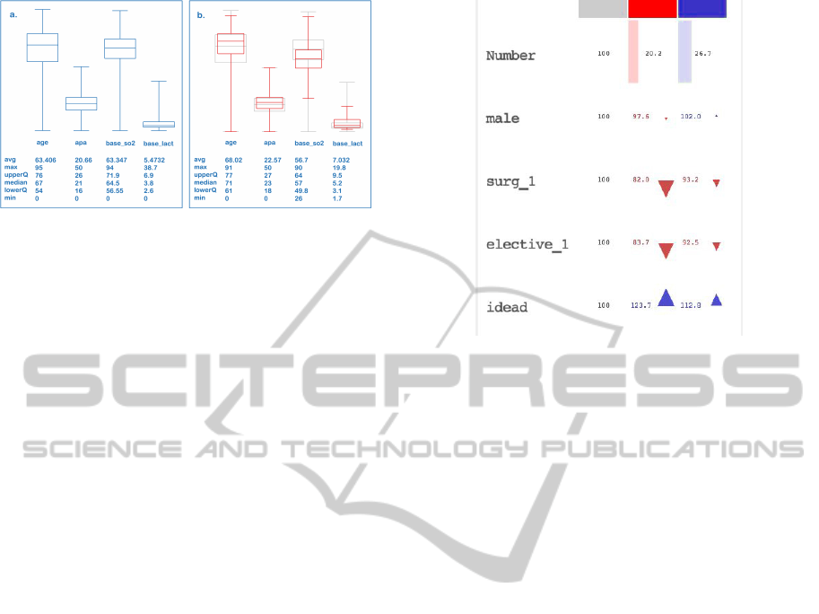
Figure 4: The newly introduced box plot view is integrated

into a CMV system. The view can show all dimensions us-

ing a relative scale, which means that all plots have the same

size although the minimum and the maximum values vary

signiﬁcantly between dimensions. a. 4 parameters depicted

using absolute scale. b. brushed items plots depicted in red

and all items in gray plots.

row shows the actual number (and/or percentage) of

selected items per brush. Each cells shows the differ-

ence between an aggregate (e.g., average, mean, etc.)

of the brush in the corresponding dimension to the

according aggregate in this dimension of the overall

dataset. This can be indicated numerically by show-

ing the calculated values directly or by the percent-

age in regard to the overall aggregate. An additional

simple triangular glyph visualizing this differences al-

lows easy and fast comparing of different selections in

many dimensions and therefore facilitates the discov-

ery of relationships between them.

4.4 The Inverse Brush

The standard brushing makes it possible to combine

several brushes using boolean operations (and, or,

not). As described above, the brushed data is then

depicted simultaneously with the context. During our

analysis session medical experts often wanted to see

the distribution of not brushed data. Note that this is

different then showing the context which represents

all data. This is also different from a simple NOT

brush. We introduce an inverse brush, a brush that

is coupled to an existing composite brush and shows

always the not selected items. In this way, it is pos-

sible that the user drills down using a combination of

several brushes, and the inverse brush follows these

selections. The system will show the context, the

brushed items and the not brushed items. If the user

interactively changes any of the brush components of

a composite brush, the inverse brush will be auto-

matically updated. The inverse brush functions in all

views, although it is most useful for summary views.

Figure 5: The brush overview shows the differences be-

tween aggregates (e.g. average, mean) of the selected sub-

sets (brushes) and of the overall dataset. Each column cor-

respond to one brush. The ﬁrst row shows the number of

selected items, further rows the aggregates by dimensions.

In this ﬁgure only percentages are shown. The arrow glyphs

allow fast perception of differences (e.g. the red brush se-

lects a subset where parameter idead is set 23,7% more of-

ten than in the overall dataset)

4.5 Supported Interaction

Besides above described views we have used par-

allel coordinates, histogram, scatter-plot, and tag-

cloud views during our analysis. All these views

are integrated in the CMV system, and they all sup-

port linking and brushing. We will brieﬂy describe

various brush types supported by those views. In

the histogram view the user can select bins that are

brushed. All records that have a particular dimension

depicted using the histogram in the range deﬁned by

the brushed bins will be highlighted. The brush can

be resized and freely moved to cover other bins. In

the scatterplot view we support a rectangular brush.

The user can select a rectangular area in the scatter-

plot and all points (patients) which are selected will

be highlighted. The brush rectangle can be moved and

resized. The parallel coordinates support axis brush-

ing, the user can brush a range on any axis. Just as in

the case of histogram, the user can resize or move the

brush, changing the range for one parameter. Finally,

the curve view supports the line brush. It is a simple

line drawn in the view. All curves that cross the line

are selected or brushed. The user can move the line or

move the line end points. Figure 6 shows four main

view types with various types of brushes.

IVAPP 2012 - International Conference on Information Visualization Theory and Applications

654

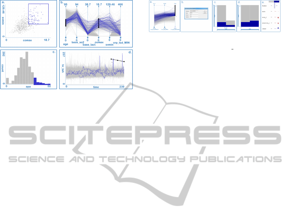
Figure 6: Various views support various types of brushing.

All items (patients) selected in one view are highlighted in

all other views. a. A rectangular brush in scatterplot selects

patients having two parameters in speciﬁed ranges. b. A

range on each axis of the parallel coordinates plot can be

selected. c. User can select neighboring bins in a histogram.

d. A simple line brush is used in the curve view. All curves

crossing the line are selected.

5 CASE STUDY

There has been increasing interest in recent years

within the critical care community in the role of serum

sodium in ﬂuid management, acid-base balance and

ICU mortality. While both high and low serum

sodium concentrations are associated with increased

mortality, therapies that rapidly change sodium con-

centrations are also associated with an increase in

mortality (Lindner et al., 2007; Rocktaeschel et al.,

2003).

We use interactive visual analysis (IVA) to ana-

lyze the data. IVA and the use of the data model sup-

porting families of curves represent a premium sup-

port tool for deep analysis, sense making and getting

insight into the data. Seeing all curves of a family

at once, seeing their aggregates and all other dimen-

sions allow experts to quickly propose a hypothesis

and check it. Our main goal is to see if there are some

hidden, still unknown indicators in the data which can

improve predictions. We investigated the effect of ab-

normal serum sodium concentrations, variability of

sodium concentration, and rapid changes in sodium

concentration on ICU mortality.

5.1 Serum Sodium Concentration:

Conﬁrming an Hypothesis

The medical experts were novice users at the begin-

ning and we started the analysis process with a well

known case. The analysis at this stage provides famil-

Figure 7: a. + b. Patients with hypernatraemia are selected

using the maximum aggregate of na tsh curves. For each

curve the maximum is computed and it is depicted using

parallel coordinates. The values above 150mmol/L are se-

lected. c. + d. The histograms shows the mortality rate for

this case (in absolute and relative scale). e. In the summary

view it can be instantly seen that the selected subset has a

higher mortality rate (parameter idead at the bottom of the

view).

iarization and reassurance to the medical team mem-

bers of the technique of interactive visual analysis, be-

fore we embarked on more complex analysis.

Normal serum concentration is typically deﬁned

as 136 − 145mmol/L. Hyponatraemia can be deﬁned

as a state where the serum sodium level is below

130mmol/L, and hypernatraemia as a state where the

serum sodium level is above 150mmol/L. Our expec-

tation is that patients with at least one recorded hyper-

natraemia or hyponatraemia have a higher mortality

rate.

To depict hypernatraemia patients, we can use a

simple line brush (user draws a line in the curve view

and all curves crossing the line are brushed) to se-

lect curves having values above 150mmol/L, or we

can compute the maximum aggregate for each curve

and depict the maximum values using, for example,

parallel coordinates. A brush on an axis of paral-

lel coordinates will be used for selection in this case

(Figure 7a). After drawing the brush with the mouse,

the user can adjust the brush limits precisely using a

brush properties dialog (Figure 7b). This is impor-

tant in cases where we want to have an exact range of

brushed data.

The histogram in Figure 7c shows the mortality

rates, the surviving cases on the left and the dead

cases on the right. To be able to visually compare the

mortality rate of the selection, we use a relative scale

on the histogram (Figure 7d), which gives the bins of

the overall data the same height and scales the high-

lighted selection data accordingly. If we had brushed

at random, or to be more precise, if we had brushed

any subset of the data with no inherent relation to

mortality, we would expect the selected bins to be the

same height. That there are relatively more cases se-

lected in the dead subset, shows that there may be an

association between hypernatraemia and higher mor-

tality rate. The same relation can be noticed instantly

in the brush overview view. In exact numbers the

overall mortality rate is 326/1447 or 22, 5%, but in

INTERACTIVE VISUAL ANALYSIS OF INTENSIVE CARE UNIT DATA - Relationship between Serum Sodium

Concentration, its Rate of Change and Survival Outcome

655

Figure 8: Exploring variability - a. Parallel coordinates

with the minimum, the maximum, and Y −SPAN aggregates

are shown. b. High variation curves are select ﬁrst (high

values for Y − SPAN, meaning a large difference between

minimum and maximum). c. The selection is reﬁned by

excluding the patients having hypo- or hypernatremia. d.

The corresponding histogram shows that mortality is higher

in those cases than in general (right dark blue bin is higher

in the relative histogram - a histogram where each bin is of

the same height used to show the ratio of brushed and non-

brushed items in each bin). e. The original curves depicted.

These patients have a higher risk, although they do not have

hypo- or hypernatremia.

patients with hypernatraemia, the mortality rate was

91/331 or 27,5%.

To compare the mortality rate (and other values)

of patients with and without hypernatraemia we used

the inverse brush to invert the selection. It shows us

a mortality rate of 21,1% in patients without hyper-

natraemia. The admission parameters such as age,

APACHE II scores, baseline serum lactate concentra-

tion and baseline venous oxygen saturation were quite

similar.

Likewise, by placing the threshold brush at

130mmol/L, we calculated the mortality of patients

with at least one recorded measurement of hypona-

traemia to be 25,2%, compared to a mortality of

20,0% in patients without hyponatraemia. Again, this

is despite very similar admission parameters. Both

these ﬁndings are consistent with conclusions drawn

using conventional methods of analysis and were ex-

pected by medical experts.

5.2 Exploring Variability of Sodium

Concentration

It is time now for more complex analysis. We ob-

served that the sodium concentration curves (na

tsh)

varied greatly for some patients and we therefore

explored whether these ﬂuctuations were associated

with mortality. To do so we computed the differ-

ence between the highest and the lowest concentra-

tion of serum sodium for each patient (i.e. the max-

imum value of the curve minus the minimum value

of the curve) and stored this as a new scalar variable

(na tsh Y − SPAN). Our data table has one additional

scalar column now.

We then used parallel coordinates (Figure 8a.) and

brushed records with the largest concentration-span

values (Figure 8b.) to compare mortality rates of pa-

tients with with high and low sodium concentration

variability.

To investigate whether high variability without

hyper- and hyponatraemia (both of course lead to high

sodium concentration variability) also increases mor-

tality we excluded patient with hypo- or hyperna-

tremia by using two subtract brushes in the parallel

coordinates view (Figure 8c.). We detect that some

patients indeed have high variability in sodium con-

centration despite never being hypo- or hypernatremic

at any time. The histogram in Figure 8d. shows the

relative mortality for those patients. It appears that

high variability in sodium concentration is associated

with mortality despite the absence of hypo- or hyper-

natremia.

5.3 Rate of Change in Serum Sodium

Concentration

A general principle in ICU ﬂuid management is

to prevent hyper- and hyponatraemia, and to avoid

rapid changes in sodium concentration. Once

hyper- or hyponatremia is established, correction

of sodium concentration is not without risks. We

therefore investigated the effects of rapid correc-

tion of sodium concentration in patients with ab-

normal sodium concentrations. To explore the ef-

fect of rate of change we computed a new variable

(na tsh 1ST DERIVATIV E) which is the ﬁrst deriva-

tive (i.e. slope of tangents) of the na tsh curve for

each patient (it is calculated by taking the difference

between two consecutive values of sodium concentra-

tion and dividing it by the time difference between the

two recordings). This is again a new column in our

dataset, a time series column where positive values

correspond to a rise in the sodium concentration and

negative values to a fall in the sodium concentration.

5.3.1 Hypernatraemia with Rapid Fall in Serum

Sodium Concentration

To select hypernatremic patients we used a curve view

showing the original na tsh data and a line brush

to select all patients with values above 150mmol/L.

Since we want to explore the cases which experience

IVAPP 2012 - International Conference on Information Visualization Theory and Applications

656

a rapid fall in sodium, we used a curve view show-

ing na tsh 1ST DERIVAT IV E. Using a line brush

we selected only curves which have values below

−3mmol/L/hour. The brushed data set showed a

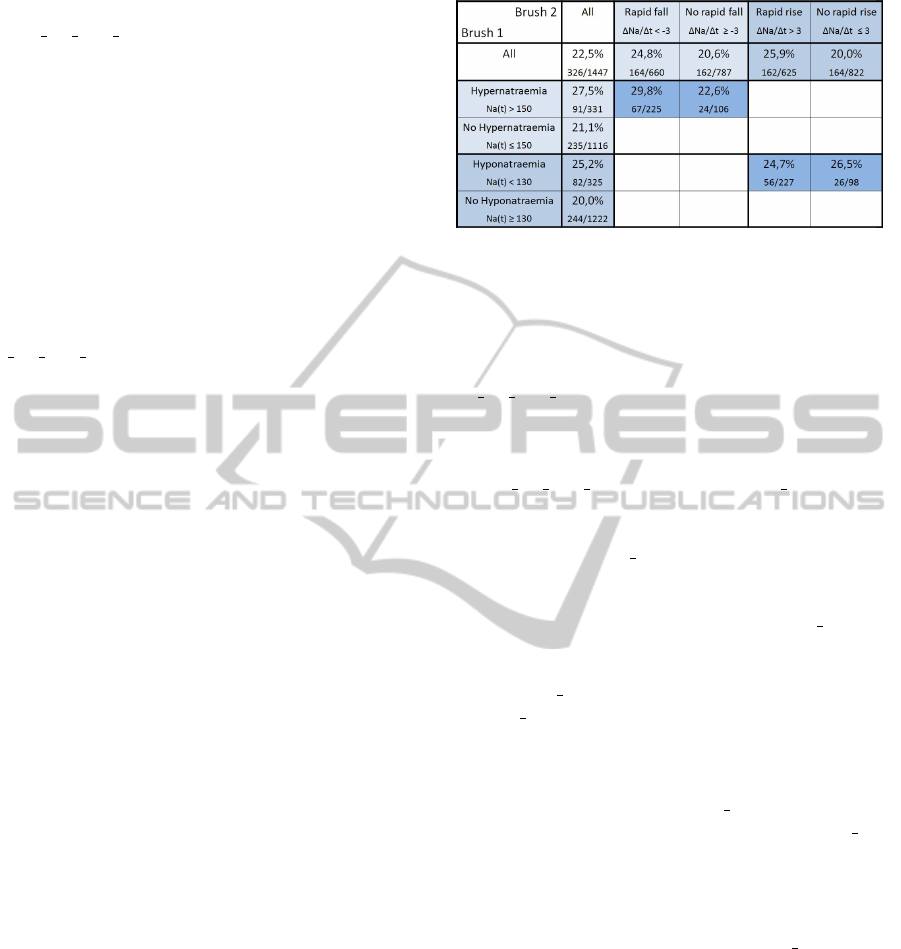
higher mortality rate of 29,8%. Interestingly, patients

with hypernatremia but without a rapid fall in sodium

concentration had a lower mortality rate (22,6%).

This suggests that hypernatraemia per se may not be

detrimental, but it may be the rapid correction that

leads to increased mortality.

That a rapid fall in sodium concentration of

over 3mmol/L/hour (regardless of hypernatraemia)

causes an increased mortality (24,8%) compared

to the mortality rate in those without (20,6%)

can be shown when applying only the brush on

na tsh 1ST DERIVATIV E.

5.3.2 Hyponatraemia with Rapid Rise in Serum

Sodium Concentration

We were also interested in the effect of a rapid in-

crease in sodium in hyponatremic patients. Using a

similar selection approach as in the previous section,

we found that a rapid rise in sodium concentration

(more than 3mmol/L/hour) is associated with a mor-

tality of 25, 9% compared to 20, 0%. In contrast to

the case with hypernatremia and rapid fall in sodium

concentration, this increased mortality with rapid rise

in sodium concentration is not pronounced in hy-

ponatraemic patients. We note that patients with a

sodium of under 130mmol/L and rise of sodium over

3mmol/L/hour have a mortality rate of 24,7% which

is quite similar (even a little lower) to patients with

hyponatraemia (25,2%), and also to patients with hy-

ponatramia and a sodium concentration rise of less

than 3mmol/L/hour(26,5%). These ﬁndings seem

to suggest that rapid rise in sodium concentration is

detrimental regardless of the concentration of sodium,

and that hyponatraemia itself is also detrimental re-

gardless of the rate of change of sodium concentra-

tion. The results are summarized in Figure 9.

5.3.3 Interactive Drill Down: A Detailed

Analysis

The next stage of analysis demonstrates the potential

of IVA to explore changes of sodium concentrations

in detail. Clinical research usually deals with popu-

lation aggregates, and time series data hereby is often

dealt by using aggregates. Interactive visual analysis

is a novel approach that medical experts are not ac-

customed to. However, the proposed data model and

the technology implemented here make it possible to

explore the data on a deeper level, as well as on the

individual patient level as on the time level.

Figure 9: The mortality rates in percent and absolute num-

bers for patients with hypernatraemia, hyponatraemia, rapid

rise and fall in sodium concentration along with interesting

combinations.

By simply making the line brush shorter on the

na tsh 1ST DERIVATIV E time series, we could eas-

ily select patients with a high rate of change in serum

sodium during speciﬁc periods of their stay at the

ICU. Figure 10 shows such an analysis. Curve views

for na tsh 1ST DERIVAT IV E and na tsh are de-

picted. Patients with a high rate of change at the be-

ginning of the ICU stay were selected (Figure 10a.).

It appears that the na tsh levels for all these patients

stabilized quite quickly after the initial ﬂuctuations.

We note visually that some patients had high initial

values, and some had low initial values of na tsh, but

the individual curves are still not distinguishable. So

we reﬁned the selection further by brushing a subset

with low na tsh values ﬁrst, and then a subset with

high na tsh (Figures 10b. and c.). Note that there is

no patient which had low values and then high values,

or vice versa. This presents a reassuring indicator that

there was appropriate ﬂuid management in these pa-

tients, leading to a normalized na tsh level.

Now we can examine a different set of na tsh

curves which had a rapid rise later in time. Fig-

ure 10d. and e. show these curves. Note the differ-

ence in curves shapes compared to the initial selec-

tion. Patients with a later rapid rise in serum sodium

had much higher oscillations in their na tsh curves

throughout their ICU stay. These oscillations may re-

ﬂect an unstable clinical course associated with more

difﬁcult ﬂuid management or they may represent a

subgroup of patients with particularly organ dysfunc-

tions such as kidney failure. Further analysis and ex-

amination of other parameters would be necessary to

conﬁrm and refute such a hypothesis.

Further investigation showed us that patients with

the highest rates of rise in sodium were those who also

suffered from severe hyponatraemia, which seemed to

suggest that rapid rises in sodium were mostly not pri-

mary problems, but reactions (either treatment or pa-

tient’s own relayed response) to low sodium concen-

INTERACTIVE VISUAL ANALYSIS OF INTENSIVE CARE UNIT DATA - Relationship between Serum Sodium

Concentration, its Rate of Change and Survival Outcome

657

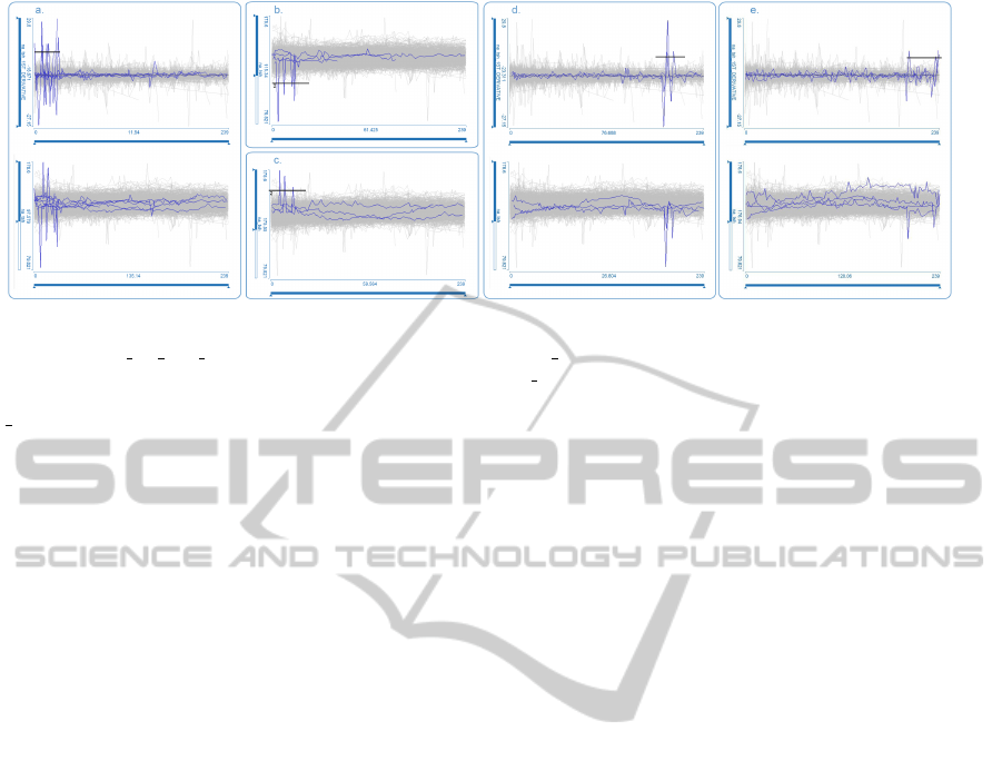
Figure 10: a. Patients which had a rapid rise in serum sodium concentration at the beginning of the ICU stay are selected by

a line brush in na tsh 1ST DERIVAT IV E (top); the corresponding na tsh curves (bottom) show patients with high and low

initial values b. and c. By applying an additional line brush at the na tsh curves we can verify that high and low initial values

correspond to different patients d. and e. Patients which had a rapid rise later in time are selected (top), the corresponding

na tsh curves (bottom) show higher oscillations.

trations. This can clearly be seen from the time series

views. Interestingly, the opposite seemed to be true

for the patients with the highest rates of fall in sodium.

The rapid falls were often the primary problem, not a

reaction to high sodium concentrations. Another ob-

servation from the drill down analysis was that pa-

tients with the lowest sodium concentrations have big-

ger oscillations on the 1st derivative time series graph

compared to patients with the highest sodium concen-

trations. These phenomen are consistent with above

described ﬁndings – hypernatraemia per se is proba-

bly well tolerated, but not rapid fall in sodium con-

centration, so patients with hypernatraemia may have

had their sodium corrected slowly. Conversely hy-

ponatraemia itself is probably harmful, so it may have

been corrected more rapidly, despite the risk of a rapid

rise in sodium concentration.

Drill down analyses as this would be very com-

plicated and almost impossible to perform using only

conventional statistical methods and aggregates. The

application of a complex data model with curves and

an interactive setup supports this discovery and explo-

ration process.

6 CONCLUSIONS

In this case study we demonstrated the usefulness of

interactive visual analysis (IVA) in analyzing a large

dataset of ICU data and helping the physicians to get

a fast and intuitive overview of the data, quickly test

hypotheses and identify relations which are worth fur-

ther examination. Furthermore, the interactive ex-

ploratory process helps domain experts to gain insight

during the analysis.

The main tasks for the interactive visualization ex-

pert reside, besides communicating the various exist-

ing visualization concepts and techniques to the do-

main experts, in providing a somehow sophisticated

data preprocessing, identifying the requirements of

the case and providing the following additional func-

tionality, tailored to the very case of application. In

our case we quickly came to the desired view conﬁg-

uration and we identiﬁed needs for improvements of

existing techniques – a curve view supporting time se-

ries with variable length and missing data, a box plot

view with multiple brushes, a summary view which

allows comparison of multiple brushes, and an easy

to use inverse brush, all fully integrated in the CMV

system.

The ICU data is a valuable source of information.

Understanding this data can contribute to improve-

ments in our comprehension of complex biological

and physiological systems, to reﬁnement of models,

for risk prediction and monitoring at both individual

and systemic levels, and ultimately to improvement in

quality of care. We have here presented how complex,

longitudinal clinical data obtained from a routinely

used clinical information system can be explored by

means of interactive visual analysis. We applied a

complex data model which, in combination with in-

teraction and various coordinated views, supports an

in-depth visual analysis. Such an analysis would not

be possible using conventional data model and con-

ventional analysis tools.

This initial exploratory study produced several in-

teresting ﬁndings. We plan to further explore these

ﬁndings and to continue to use and improve the inter-

active visual analysis tool to facilitate the analyses of

complex clinical datasets. The feedback from domain

experts is very positive, and this study resulted in an

on-going collaboration. There are many aspects we

IVAPP 2012 - International Conference on Information Visualization Theory and Applications

658

have not tackled yet, and the amount of data available

represents a huge potential for future research, both,

in visualization and in the medical domain.

ACKNOWLEDGEMENTS

The authors thank St. Thomas Hospital for data and

Zoltan Konyha for converting the data ﬁrst time. Part

of this work was done in the scope of the K1 program

at the VRVis Research Center (http://www.VRVis.at).

REFERENCES

Aigner, W., Miksch, S., M

uller, W., Schumann, H., and

Tominski, C. (2007a). Visual methods for analyzing

time-oriented data. IEEE Transactions on Visualiza-

tion and Computer Graphics, pages 47–60.

Aigner, W., Miksch, S., M

uller, W., Schumann, H., and

Tominski, C. (2007b). Visualizing time-oriented

data–A systematic view. Computers & Graphics,

31(3):401–409.

Aris, A., Shneiderman, B., Plaisant, C., Shmueli, G.,

and Jank, W. (2005). Representing unevenly-spaced

time series data for visualization and interactive ex-

ploration. Human-Computer Interaction-INTERACT

2005, pages 835–846.

Bade, R., Schlechtweg, S., and Miksch, S. (2004). Con-

necting time-oriented data and information to a co-

herent interactive visualization. In Proceedings of the

SIGCHI conference on Human factors in computing

systems, pages 105–112. ACM.

Gan, H., Matkovic, K., Ammer, A., Purgathofer, W., Ben-

nett, D., and Terblanche, M. (2011). Interactive visual

analysis of a large icu database: a novel approach to

data analysis. Critical Care, 15(Suppl 1):P135.

Gresh, D., Rabenhorst, D., Shabo, A., and Slavin, S. (2002).

Prima: A case study of using information visualiza-

tion techniques for patient record analysis. In Visual-

ization, 2002. VIS 2002. IEEE, pages 509–512. IEEE.

Hochheiser, H. and Shneiderman, B. (2002). Visual queries

for ﬁnding patterns in time series data. University of

Maryland, Computer Science Dept. Tech Report, CS-

TR-4365.

Hochheiser, H. and Shneiderman, B. (2004). Dynamic

query tools for time series data sets: timebox widgets

for interactive exploration. Information Visualization,

3(1):1–18.

Knaus, W., Wagner, D., Draper, E., Zimmerman, J.,

Bergner, M., Bastos, P., Sirio, C., Murphy, D.,

Lotring, T., and Damiano, A. (1991). The apache

iii prognostic system. risk prediction of hospital mor-

tality for critically ill hospitalized adults. Chest,

100(6):1619–36.

Knaus, W. A., Draper, E. A., Wagner, D. P., and Zimmer-

man, J. E. (1985). APACHE II: a severity of dis-

ease classiﬁcation system. Critical care medicine,

13(10):818–829.

Konyha, Z., Matkovic, K., Gracanin, D., Jelovic, M., and

Hauser, H. (2006). Interactive visual analysis of fami-

lies of function graphs. IEEE Transactions on Visual-

ization and Computer Graphics, 12(6):1373.

Lindner, G., Funk, G.-C. C., Schwarz, C., Kneidinger, N.,

Kaider, A., Schneeweiss, B., Kramer, L., and Druml,

W. (2007). Hypernatremia in the critically ill is an in-

dependent risk factor for mortality. American journal

of kidney diseases : the ofﬁcial journal of the National

Kidney Foundation, 50(6):952–957.

McGill, R., Tukey, J. W., and Larsen, W. A. (1978). Vari-

ations of box plots. American Statistician, 32(1):12–

16.

Plaisant, C., Lam, S., Shneiderman, B., Smith, M., Rose-

man, D., Marchand, G., Gillam, M., Feied, C., Han-

dler, J., and Rappaport, H. (2008). Searching Elec-

tronic Health Records for temporal patterns in patient

histories: A case study with Microsoft Amalga. In

AMIA Annual Symposium Proceedings, volume 2008,

page 601. American Medical Informatics Association.

Plaisant, C., Milash, B., Rose, A., Widoff, S., and Shneider-

man, B. (1996). LifeLines: visualizing personal histo-

ries. In Proceedings of the SIGCHI conference on Hu-

man factors in computing systems: common ground,

pages 221–227. ACM.

Plaisant, C., Mushlin, R., Snyder, A., Li, J., Heller, D.,

and Shneiderman, B. (1998). LifeLines: using vi-

sualization to enhance navigation and analysis of pa-

tient records. In Proceedings of the AMIA Symposium,

page 76. American Medical Informatics Association.

Powsner, S. M. and Tufte, E. R. (1994). Graphical summary

of patient status. Lancet, 344(8919):386–389.

Roberts, J. (2007). State of the art: Coordinated & mul-

tiple views in exploratory visualization. In Coordi-

nated and Multiple Views in Exploratory Visualiza-

tion, 2007. CMV’07. Fifth International Conference

on, pages 61–71. IEEE.

Rocktaeschel, J., Morimatsu, H., Uchino, S., and Bellomo,

R. M. (2003). Unmeasured anions in critically ill pa-

tients: Can they predict mortality? Critical Care

Medicine, 31(8):2131–2136.

Shneiderman, B. (2002). The eyes have it: A task by data

type taxonomy for information visualizations. In Vi-

sual Languages, 1996. Proceedings., IEEE Sympo-

sium on, pages 336–343. IEEE.

Trobec, R., Matkovic, K., Skala, K., Depolli, M., and Av-

belj, V. (2008). Visual Analysis of Heart Reinervation

after Transplantation. In Proceedings of the MIPRO

2008.

Tukey, J. W. (1977). Exploratory data analysis. Addison

Wesley.

Wang, T., Plaisant, C., Quinn, A., Stanchak, R., Murphy, S.,

and Shneiderman, B. (2008). Aligning temporal data

by sentinel events: discovering patterns in electronic

health records. In Proceeding of the twenty-sixth an-

nual SIGCHI conference on Human factors in com-

puting systems, pages 457–466. ACM.

INTERACTIVE VISUAL ANALYSIS OF INTENSIVE CARE UNIT DATA - Relationship between Serum Sodium

Concentration, its Rate of Change and Survival Outcome

659