
A NOVEL STATE PARAMETRIZATION FOR STEREO-SLAM
Arne Petersen and Reinhard Koch
Multimedia Information Processing, Christian-Albrechts-University, Hermann-Rodewald-Str. 3, D-24118 Kiel, Germany
Keywords:
SLAM, SfM, Stereo, Linear Estimation.
Abstract:
This paper proposes a novel parametrization for probabilistic stereo SLAM algorithms. It is optimized to
fulfill the assumption of Gaussian probability distributions for system errors. Moreover it makes full use of the
contraints induced by stereo vision and provides a close to linear observation model. Therefore the position
and orientation are estimated incremetally. The parametrization of landmarks is chosen as the landmarks
projection in the master camera and its disparity to the projection in the slave camera. This way a minimal
parametrization is given, that is predestinated for linear probabilistic estimators.
1 INTRODUCTION
The task of visual Simultaneous Localization And
Mapping (SLAM) is to keep track of the position and
orientation, pose for short, and the environment map
of a vision system. The environment map mostly con-
sists of so called landmarks that represent parts of
the map that can be observed using cameras. Mod-
els for the observations of the environment and for
most SLAM methods the systems motion are used to
estimate this parameters.
After the first SLAM systems have been devel-
oped in the mid 1980’s, see (Brooks, 1985) and
(Crowley, 1989), algorithms for SLAM have been
studied intensely, e.g. see (Leonard and Durrant-
Whyte, 1992), (Dissanayake et al., 2001), (Paz et al.,
2008), (
˙
Imre and Berger, 2009). This is due to
its applicability to autonomous navigation and auto-
matic environment field mapping. These tasks be-
come increasingly important as automatization using
autonomous vehicles is applied to more and more
areas. This includes airborne and ground (Lemaire
et al., 2007) as well as underwater (Hildebrandt and
Kirchner, 2010) vehicles.
Many solutions to the SLAM problem use the
Kalman Filter (KF) introduced by Kalman in 1960
(Kalman, 1960). This estimator is used due to its low
computational costs despite its drawback in estimat-
ing non linear processes. Thus, the choice of state
parametrization is crucial to keep the filter state and
reliability (covariance matrix) estimation consistent.
It has to be chosen in a way that allows for close to
linear system models (prediction and observation) and
meets the Gaussian noise assumption made by the KF.
Therefore a new parametrization for the parameters to
be observed by a stereo vision system is introduced,
that uses the stereo correspondences for the respec-
tive landmarks and a local navigation frame. The pro-
jection of the landmark into the left (master) stereo
camera and its disparity to the right (slave) camera
represent its position in 3D space. By this means the
landmarks are described relative to the actual system
pose. For this representation the assumption of zero
mean Gaussian noise for its errors is met. The model
proposed in this article enables linear least squares es-
timators like KFs to determine consistent state and re-
liability information.
Even though stereo camera systems are limited by
the stereo baseline in direct depth measurements, their
use is helpful for many reasons. The limitation due to
the baseline can be reduced by increasing image res-
olution and using models relating stereo images over
time (see sec. 3.2). Moreover monocular reconstruc-
tions have the drawback of a global scale ambiguity,
see (Hartley and Zisserman, 2003). This ambiguity
also causes a drift in the scale due to error accumula-
tion. Since the reconstruction using stereo is metric,
sensors like accelerometers can be incorporated with-
out estimating the reconstruction scale.
Beside synthetic test experiments are made us-
ing a dataset provided by the Rawseeds Project
(www.rawseeds.org, see (Ceriani et al., 2009) and
(Bonarini et al., 2006)). It delivers the sensor data
(stereo camera images and IMU data) from a wheel
driven robot system navigating in a plane. Moreover
ground truth information is available for the whole
144
Petersen A. and Koch R..
A NOVEL STATE PARAMETRIZATION FOR STEREO-SLAM.
DOI: 10.5220/0003844601440153
In Proceedings of the International Conference on Computer Vision Theory and Applications (VISAPP-2012), pages 144-153
ISBN: 978-989-8565-04-4
Copyright
c
2012 SCITEPRESS (Science and Technology Publications, Lda.)

covered trajectory. This way the pose estimation
along with its consistency to the estimated covari-
ance can be verified. As will be shown, the proposed
method is able to reliably estimate both entities con-
sistently even for large datasets.
Following this introduction previous work in the
field visual SLAM is presented and some prerequi-
sites are given. After the description of the used mod-
els an comparison with state of the art methods is
done and some experiments are discussed.
2 PREVIOUS WORK
Various kinds of estimators have been designed to
solve the task of SLAM. These range from direct esti-
mation of quadrifocal tensors (Hildebrandt and Kirch-
ner, 2010) and particle filters (
˙
Imre and Berger, 2009)
to extended Kalman Filters (Schleicher et al., 2007).
Nevertheless the most commonly used estimators are
based on the famous KF. This is due to the fact that
SLAM usually requires real time performance and the
simple integration of multiple sensors, allowing for
compensating the errors induced by the different sen-
sors types. The ability to not only estimate the system
state but also information on the estimations reliabil-
ity is another reason for its popularity.
As stated the KF is error-prone when non linear
models are used. Because of this the use of more ad-
vanced versions of the KF have been studied. The
advantages and drawbacks of these filters have been
analyzed in (Lefebvre et al., 2004). Their applica-
tions to SLAM include beside others the unscented
Kalman Filter (S
¨
underhauf et al., 2007) as well as it-
erated sigma point Kalman Filters (Song et al., 2011).
Such approaches try to overcome the drawbacks of
non linear models by using estimators more robust in
such cases. Thus the non linearities themselves are
not eliminated but more complex algorithms are used.
This results in increased computational costs and thus
less applicability to real time demands.
Apart from the used estimators the solutions to the
SLAM problem differ in the representation of land-
marks. For visual SLAM the so called Inverse Depth
(ID) representation is used mostly, e.g. see (Civera
et al., 2008),(S
¨
underhauf et al., 2007). There a land-
mark is represented by the position of the camera
from where the point was observed first, the direction
to the 3D point and its inverse distance to the cam-
era center. A drawback of this parametrization is, that
is uses a 6 dimensional representation. Since a land-
mark (point in 3D-space) only has 3 degrees of free-
dom (DOF), it is over parametrized. Thus, ambigui-
ties in the estimation can arise, since points initialized
from the same camera end up with different camera
positions. (Civera et al., 2008) have shown, that in ID
the error propagation for depth is linear under certain
assumptions. Nevertheless the models include inverse
tangent and normalization functions resulting in non
linearities not analyzed by Civera et al..
Since the ID parametrization for landmarks suf-
fers from inconsistent covariance estimation for short
distances, (Paz et al., 2008) discuss a combination
of representations. For their stereo SLAM system
they partition landmarks in far away and nearby
landmarks. For far points ID is used, and the 3D
Euclidean Space (ES) for nearby points. This im-
proves the estimation of landmarks and the system
pose, but as can be seen in their evaluation, the
parametrization still has problems covering the true
error distribution for reconstructed 3D points.
Due to the above mentioned benefits provided by
stereo camera systems, many stereo SLAM systems
have been developed, see (Paz et al., 2008), (Hilde-
brandt and Kirchner, 2010), (Schleicher et al., 2007).
The latter propose a system solely based on wide an-
gle stereo cameras and a two stage algorithm. They
create small local maps and detect close loops us-
ing SIFT-fingerprints. In (Hildebrandt and Kirchner,
2010) a system is discussed, that uses an IMU aided
estimation of the quadrifocal tensor.
In (Sol
´
a et al., 2007) the authors claim, that us-
ing two independent cameras outperforms stereo rigs.
In fact, they propose a combination of monocular and
stereo vision resulting in improved estimation. Since
this is a combination of both models, this approach
can be used to fuse most monocular and stereo mod-
els. In (Herath et al., 2006) a representation similar to
the one presented here, has been proposed for obser-
vation models. In contrast to our work they do not use
this for modeling landmarks in the SLAM system. It
was shown, that such observation models undergo a
Gaussian noise assumption.
Our Contribution. The main contribution of this
paper is to introduce a novel parametrization for land-
marks optimized for stereo SLAM algorithms using
image Points and Disparities (PD). This parametriza-
tion allows a minimal representation of a 3D land-
mark, that is, 3 parameters are used for the 3 DOF.
On the one hand this parametrization outperforms the
one in Euclidean 3-space by matching the Gaussian
noise distribution much better. On the other hand
compared to inverse depth it reduces the number of
variables to be estimated from 6 to 3 per landmark.
Moreover the resulting observation model is kept sim-
ple and the landmarks can be initialized accurately in
position and uncertainty.
A NOVEL STATE PARAMETRIZATION FOR STEREO-SLAM
145

Because of the reduced parameter size and the sim-
ple observation model compared to inverse depth the
computational costs are decreased for SLAM sys-
tems. Thanks to the new model the equations used
for estimation can be accurately linearized using their
analytical derivatives. This again reduces the com-
putational effort. As will be shown, the proposed
parametrization is capable of improving the estimated
poses covariance matrix. Thus, in contrast to ID
parametrization the computed global position and ori-
entation are consistent with the estimated variances.
Hence, the proposed parametrization outperforms the
ID by improving consistency and computational ef-
fort.
3 PREREQUISITES
In this section the notation used throughout this paper
is introduced and some prerequisites needed for the
proposed algorithms are given.
3.1 Iterated Kalman Filters
The description of the iterated extended KF (IEKF)
used in this paper is based on the EKF in (Welch and
Bishop, 2006). Since a detailed description of the KF
is out of the scope of this paper we refer to them. For
simplicity the notation introduced there will be used
to augment the proposed extended KF by iterative lin-
earization. Since the prediction is done as in the EKF
only the update step is described here.
An additional index is introduced to the Jacobian
H
k
of the used measurement models, denoted as h.
H
(ν)
k
refers to the ν
th
iteration step and the respective
state estimation p
(ν)
k
, that is:
H
(ν)
k
=
∂h(p)
∂p
p=p
(ν)
k
(1)
Let l
k
the observation for the k
th
time step and P
l
k
its
covariance matrix. Using the state prior as iteration
start p
(0)
k
and the respective covariance matrix P
−
k
the
ν
th
iteration is defined by:
p
(ν)
k
= p
(0)
k
+ K
(ν−1)
k
·z
(ν−1)
k
(2)
K
(ν)
k
= P
−
k
H
(ν)
k
H
(ν)
k
P
−
k
H
(ν)
k
T
+ P
l
k
−1
(3)
z
(ν)
k
= l
k
− h
p
(ν)
k
− H
(ν)
k
·
p
(0)
k
− p
(ν)
k
(4)
The iteration process is continued until ν reaches
a certain maximum or
p
(ν)
k
−p
(ν−1)
k
2
falls beneath a
x
s
m
d
x
m
b
s
X
Y
Z
s
m
s
'
m
'
X
R,t
T(m,s,s')
T(m,s,m')
Figure 1: Hardware setup: master and slave camera (m, s)
and transformed system (m
0
, s
0
). TFT T and transformation
R,t.
given threshold. The covariance matrix P
+
k
for the
finally estimated state is afterwards computed by:
P
+
k
=
I − K
(ν)
k
H
(ν)
k
P
−
k
(5)
This equation can be derived directly using the deriva-
tion for the Gauß-Markov-Models and the Kalman
Filter in (McGlone et al., 2004), chapter 2.2.4. Using
this update equations the error incorporated by non
linear observation models can be minimized. How-
ever, this applies only to models where all non lin-
earities of the system are observed at the same time.
In this case the IEKF outperforms even the unscented
or sigma point Kalman Filters (see (Lefebvre et al.,
2004) for details).
3.2 Stereo Vision and Trifocal Tensor
The stereo camera system is made up of 2 cameras,
the master camera m and the slave camera s, differing
only in a translation t
ms
= (
b 0 0
)
T
with baseline b.
Projecting a 3D point X into both cameras, 2 points
in the respective image planes result x
m
and x
s
. Using
x(i) to refer to the i
th
component of x the disparity is
d = x
m
(1)−x
s
(1). Since b > 0 and all observed points
are in front of the cameras, d > 0 holds for perfect
correspondences x
m
and x
s
. In projective geometry
d = 0 holds for points at infinity. These entities and
the used coordinate system are visualized in figure 1.
Let P
1
, P
2
and P
3
the projections for 3 different
cameras. Projecting a 3D-point X into the image
planes of the 3 cameras results in corresponding 2D-
points x
1
, x
2
and x
3
. The TriFocal Tensor (TFT, see
(Hartley and Zisserman, 2003)) T can be used to map
2 corresponding points to the third in the respective
camera, that is:
T (P
i
, P
j
, P
k
, x
i
, x
j
) = x
k
(6)
for all permutations of i, j, k, see figure 1. This is es-
pecially useful when dealing with stereo camera sys-
tems. It can be used for estimation of transformations
between stereo rigs without triangulation of X . When
VISAPP 2012 - International Conference on Computer Vision Theory and Applications
146

the system m,s is transformed to m
0
,s
0
the two TFTs
can be computed. Since the transformations m → s
and m
0
→ s
0
are known, only one transformation con-
strained by both TFTs has to be estimated.
4 SLAM USING PD
Since the task of SLAM integrates map building, the
landmarks have to be modeled as parameters for es-
timation. As stated in section 2 mainly two repre-
sentations of 3-space points are used. The most sim-
ple uses the 3 parameters of Euclidean 3-space (ES)
and the other one is ID, having 6 DOF. The former
uses a minimal set of parameters but hardly fulfills
the assumption of Gaussian noise. The latter is over
parametrized but has proven to fit a normal distribu-
tion for its depth errors under certain assumptions. A
drawback for ID is the non linearity caused by using
spherical coordinates for ray parametrization.
4.1 PD Parametrization
The landmark parametrization proposed in this paper
uses a minimal set of parameters, relates the image
measurements to the system state nearly linear and
undergoes a Gaussian error distribution.
The state to be estimated includes the systems
pose as well as its landmarks. Therefore a represen-
tation for landmarks and poses has to be used, well
suited to the needs of linear estimators.
The PD (point-disparity) representation proposed
in this article codes a position in 3-space as its projec-
tion to the stereo system. Since the stereo calibration
is assumed to be known, the projection to the mas-
ter camera x
m
and its 1-dimensional displacement d
to the projection to the slave camera (see figure 1) is
sufficient. This results in a representation
X
k
=
x
m,k
d
k
(7)
using 3 DOF, which is minimal for a point in 3-space.
Here the index k is needed since the representation is
relative to the actual pose and thus, dependent on the
time step k.
The parametrization used for estimation of the
pose π
k
consists of the 3-space position increment
t
k
of the master camera and the orientation incre-
ment ∆φ
k
in Euler angles relative to the last estimated
pose. Thus, the pose describes the transformation be-
tween the past and actual pose in the global coordi-
nate frame. For the ES and ID estimation the pose
is given relative to the global coordinate system de-
fined by the initial camera pose. Thus, for N land-
marks X
1
, . . . , X
N
in the respective representation ES,
ID and PD the parameter vector to be estimated is:
p
k
=
π
k
X
1
k
.
.
.
X
N
k
(8)
For the representation in ES both parts are inde-
pendently represented in the same global reference
system. By this, the observation model relates the ob-
servations to the landmarks and the actual global pose
directly. For the ID the poses of past time-steps are
used to represent landmarks. Thus, the observations
relate to landmarks, the actual and the past poses. The
PD representation relates the observations to the dif-
ference of the actual and the past pose as well as the
landmarks. Comparing this relations, the estimation
using ES and PD representations includes parameters
of actual poses only, leaving the estimation steps in-
dependent over time. For the ID representation actual
and past poses are estimated. Moreover, in PD each
estimation step relates only the actual and last pose.
That is, it is incremental and correlations in time (i.e.
drift) don’t contradict the unbiasedness of KF models.
4.2 Observation Model
In the following the time index k is omitted for better
readability. For observing the PD landmarks, stereo
correspondences are used. That is a landmark X
i
is
mapped to 2 image points y
i
m
in the master camera and
y
i
s
in the slave camera respectively. The landmark de-
scribes the respective stereo correspondence relative
to the previously estimated pose. Using the trifocal
tensor, y
i
m
and y
i
s
can be predicted using the initial es-
timate p
0
, possibly including a guess for the systems
movement as in KF prediction. This is implemented
in the measurement models h
m
and h
s
. Thus, the ob-
servations and the measurement model are:
l =
y
i
m
y
i
s
i
and h (p) =
h
m
π, X
i
h
s
π, X
i
i
(9)
Let R the rotation matrix for the differential orien-
tation ∆φ. Further let R
g
be the rotation matrix cor-
responding to the global orientation (integrated over
all preceding R) for the initial parameters guess p
0
.
Using this notation the landmarks projection can be
predicted in homogeneous coordinates via the TFT,
see (Hartley and Zisserman, 2003):
Y
i
m
= R
T
b
x
i
m
1
− d
i
R
T
g
t
(10)
for the master camera. The disparity is predicted us-
ing b·d
i
·
Y
i
m
(3)
−1
. Thus, the prediction for the cor-
A NOVEL STATE PARAMETRIZATION FOR STEREO-SLAM
147

respondence i ends up with:
h
m
(p) =
1
Y
i
m
(3)
Y
i
m
(1)
Y
i
m
(2)
(11)
and
h
s
(p) =
1
Y
i
m
(3)
Y
i
m
(1) − b·d
i
Y
i
m
(2)
(12)
Note that this model and the landmark
parametrization allow disparities of 0. This way, the
proposed models can be easily extended to include
points at infinity to improve orientation estimation.
The simplicity of this observation model enables
the determination of its analytical derivatives. Thus,
a precise linearization can be done and there is no
need for a time consuming numerical computation
of the Jacobians required for linear estimation.
Compared to the models used for projecting points
represented in ID (see (Civera et al., 2008)) this is an
advancement. For them the computation of the view
ray b (
x
i
m
(1) x
i
m
(2) 1
)
T
is replaced by a conversion from
spherical to Euclidean coordinates.
4.3 Initialization and Estimation
When a landmark is observed first as y
m
and y
s
, it has
to be incorporated into the system state. For the PD
representation this can be achieved by:
x
m
(1) = y
m
(1) d = y
m
(1) − y
s
(1)
x
m
(2) =
1
2
(y
m
(2) + y
s
(2))
In contrast to the initialization of ID-landmarks (con-
version from Euclidean to spherical coordinates and
depth determination by vector norm) this is strictly
linear, so that the assumed measurement noise can
be directly propagated to the landmarks covariance.
As for most pose estimators the systems initial posi-
tion and orientation are used as the world coordinate
frame.
To estimate the pose for time k the IEKF from sec-
tion 3.1 is applied using the given observation model.
After the actual pose has been estimated, the pose and
landmarks have to be transferred to the new camera
body frame. Therefore the landmarks are mapped to
the new camera view using the same model as for
the observation. That is, the projections to the new
master camera and the respective disparities are pre-
dicted. Afterwards the position and orientation incre-
ments are added to the global pose and set to 0. Ac-
cording to this, the parameters covariance matrix is
computed using linear error propagation.
The global poses are computed by integrating the
position and orientation increments estimated over
time. This also applies to the estimated covariances.
This way the estimated entities correspond to a ran-
dom walk process. By this, the standard deviation
bounds the global poses even though a drift is incor-
porated. Another advantage of this incremental esti-
mation is, that loop closes, applied to sub tracks of the
estimated trajectory, directly effect new poses. Build-
ing the integral over the state sequence also updates
subsequent poses. Thus, partial adjustments improve
the complete trajectory estimation.
The global landmarks are computed using their lo-
cal representation and the global poses. For each view
a 3-space point is created and these are averaged over
all views. Since their representation is as seen from
the respective pose, this can be done incrementally.
This way the information on this landmark from all
views is exploited. For advanced landmark model-
ing particle casts can be performed to create empirical
probability distributions for all landmarks and views.
Therefore the estimated covariance matrices for the
landmarks and poses can be used to generate the re-
spective particle cloud.
5 PERFORMANCE ANALYSIS
In this section analysis and comparison of the pro-
posed and state of the art methods are carried out.
Therefore the landmarks parametrizations for ES, ID
and PD and the estimations qualities are compared.
For the evaluation of landmark initialization two
different tests have been performed. At first the land-
marks represented in ES, ID and PD respectively are
generated using a particle cast from stereo correspon-
dences. Therefore, the ground truth correspondences
are disturbed by Gaussian noise. The resulting pa-
rameter clouds represent the parametrizations empir-
ical probability distributions, when initialized using
stereo features. Thereby the assumption of Gaussian
noise for the respective representation can be vali-
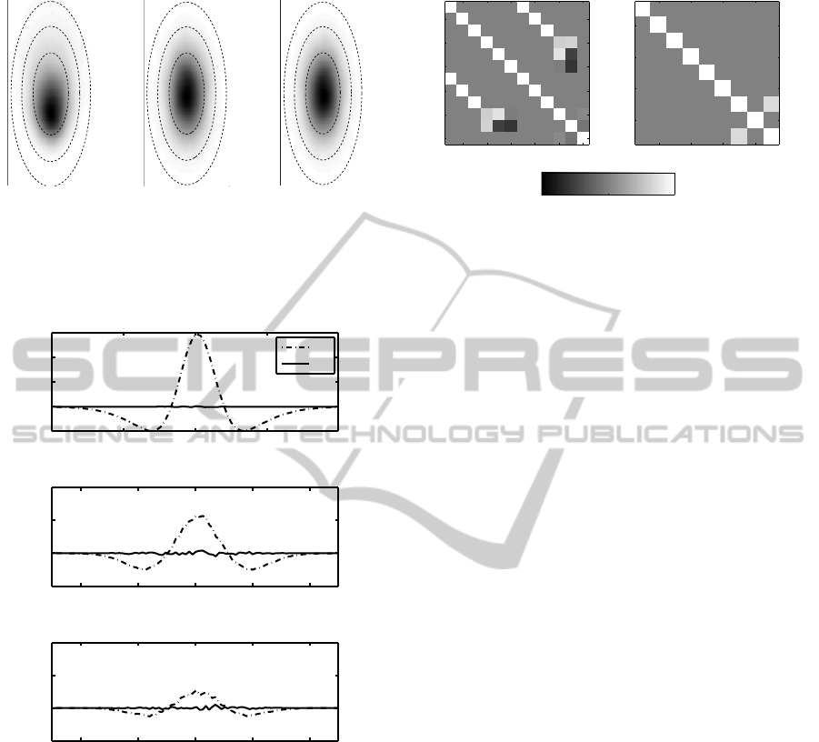
dated when used for stereo vision systems. In fig-
ure 2 the accordant distributions are visualized. As
can be seen, the ID and PD undergo a Gaussian error
distribution. In contrast, ES obviously violates this
assumption for large distances. For close landmarks
all three parametrizations fit the Gaussian noise quite
well.
For the second test of initialization an ID and a PD
landmark are generated from a perfect stereo corre-
spondence using the given initialization methods. Af-
terwards noise with covariance C
2D
is added to the
stereo correspondences and a 3-space cloud is gen-
erated via particle cast. Following this, covariances
C
ID
and C
PD
are computed from C
2D
using the Ja-
cobians of the initialization functions. Normal dis-
VISAPP 2012 - International Conference on Computer Vision Theory and Applications
148
−0.5 0 0.5
30
50
70
90
ES YZ
−0.01 0 0.01
0.005
0.01
0.015
0.02
0.025
ID: β/ID
−0.01 0 0.01
0.01
0.02
0.03
0.04
0.05
PD Y/Disp
Figure 2: Empirical probability distributions and propa-
gated covariance ellipses in parameter space. Units, ES:
baselines ID: radiants,fractions of baselines PD: normalized
pixels.
−0.02 −0.01 0 0.01 0.02
−5
0
5
10
x 10
−3
ε
p
x
distance 100 baselines
−0.02 −0.01 0 0.01 0.02
−5
0
5
10
x 10
−3
ε
p
x
distance 5 baselines
−0.04 −0.02 0 0.02 0.04
−0.02
0
0.02
0.04
0.06
x
ε
p
distance 1 baseline
ID
PD
Figure 3: Difference between empirical and ground truth
probability distributions for reprojection with different
point-camera distances. X-axis marks normalized pixel co-
ordinates and y-axis the error of probability ε
p
.
tributed noise is added to the ground truth landmarks
in ID/PD domain according to C
ID
and C
PD
. Finally
the 3-space, ID-space and PD-space clouds are re-
projected into the image and their distributions are
compared. As in the former evaluation the distribu-
tion generated by stereo correspondences is used as
ground truth for validation. As can be seen in figure
3, the deviation between the true error distribution and
the one for ID is much higher compared to the one
of PD, which is negligible. Moreover, it increases
strongly with decreasing point-camera distance. A
Correlation matrix ID
2 4 6 8 10 12
2
4
6
8
10
12
Correlation matrix PD
2 4 6 8
2
4
6
8
−1 0 1
Figure 4: Initial ID/PD correlation matrices for pose and a
single landmark. Left ID: component 1-6 pose, 7-12 land-
mark (7-9 pos., 10-12 ray/idepth). Right PD: 1-6 pose, 7-9
landmark (7,8 master pixel, 9 disparity).
similar effect was observed by (Paz et al., 2008) for
the reconstruction of 3-space points from ID. This is
due to the violation of the assumption made in (Civera
et al., 2008), that the view angle between the first ob-
servations (i.e. initial and second) of the ID feature
have to be small. From this it can be concluded, that
the measurement model for PD yields a more consis-
tent update prediction, i.e. in case of close features.
A drawback of the ID parametrization is that the
poses position is used as the landmarks reference po-
sition. This way a correlation equaling 1 is intro-
duced (see figure 4, components 1-3 and 7-9 respec-
tively). Because of this the systems covariance ma-
trix is singular after initialization. This remains when
no prediction noise is added for subsequent estima-
tions. Moreover the covariance will be closer to sin-
gular the less noise is added. On the one hand, this
leaves the ID unapplicable for general least squares
estimators and according statistical analysis, as are
described in (Petersen and Koch, 2010). On the other
hand, the matrix might loose positive semidefinite-
ness (required for covariance matrices) due to numer-
ical issues. Because the PD landmarks initialization
is uncorrelated with the system pose, no 1 : 1 correla-
tions occur.
To verify the consistency and quality of pose esti-
mation, different trajectories have been estimated us-
ing synthetical data. Therefore position and orien-
tation increments are generated and summed up to
global poses. For every trajectory step an estimation
was performed. For the pose prediction the ground
truth increments were used disturbed with Gaussian
noise according to the assumed prediction uncertainty
(prediction of P
−
k
in equation 5). When initializ-
ing landmarks from stereo correspondences dispari-
ties/depths smaller zero might occur (points behind
camera). This can be circumvented by omiting points
with disparity smaller three times the observations
A NOVEL STATE PARAMETRIZATION FOR STEREO-SLAM
149

Table 1: RMS, absolute error (baselines/deg.) and [1, 2, 3] σ inliers in %. Averaged over 100 randomly generated trajectories
with 1000 estimations each. Avg. landmarks 35, translation 3.5 baselines, orientation change 14.5 degrees per time step.
Stdev prediction noise 0.7 baselines, 3 degrees. Stdev observation noise 0.005 normalized pixels (∼ 3 px for 500
2
px images).
position orientation
RMSE mean 1σ [%] 2σ [%] 3σ [%] RMSE mean 1σ [%] 2σ [%] 3σ [%]
x 1.49 1.18 4.8 8.5 12 1.6 1.26 6.25 11.5 16.6
ES y 1.28 1.02 5.7 10.6 14.8 1.64 1.29 6.17 11.4 16.4
z 1.54 1.23 5.1 9.1 12.7 1.6 1.24 6.93 12.6 18
x 0.88 0.71 37.2 65.3 82.9 0.9 0.72 23.6 43.6 58.8
ID y 0.9 0.72 37.2 65.5 82 0.93 0.74 22.1 41.4 56.8
z 0.94 0.76 39.2 66.2 82.3 0.93 0.75 19.3 36.2 49.7
x 1.13 0.9 62.4 88.9 97 1.2 0.94 83.5 99.3 ∼100
PD y 1.06 0.84 65.2 91.2 98.1 1.25 0.99 82.1 99.3 ∼100
z 1.27 1.02 58.7 86.8 96.1 1.2 0.94 85.6 99.5 ∼100
pixel noise. This is done to keep the analysis compa-
rable for all systems. For error evaluation, the results
have been averaged over 100 test runs.
As can be seen in table 1 the root mean
square (RMSE) and mean absolute error for PD is
slightly increased compared to ID. In contrast, the
ES parametrization obviously suffers from imprecise
landmark estimation for long term applications. An-
other advantage of ID and PD estimation compared to
ES is, that they are much less biased. This was con-
cluded from the fact, that estimating a trajectory par-
allel to a planar point cloud results in a strong bias
along the direction to the cloud for ES. The same
results apply for the RMSE and mean error of land-
marks after the final estimation. As stated in section
4.3, the PD landmarks estimation is thought to be av-
eraged over time using particle casts. In this case the
error can be reduced by 66% compared to ID at the
cost of increased computational effort.
In table 1 the inliers for the 1,2 and 3 σ-confidence
interval are listed. An inlier is defined by being inside
a given confidence interval. That is, for the 1σ, 2σ and
3σ confidence area the expected percentage of inliers
is 69%, 95% and >99% respectively. As can be seen,
the ES and ID estimation are inconsistent. In con-
trast to this, the PD estimation stays consistent for the
orientation even for long term runs, in this case 1000
estimations. The PDs position variance is improved
considerably but still shows small inconsistencies of
a few percent. This is due to the time correlations
of position increments being much higher compared
to orientation. To compensate this, the consistency
method for joint covariances discussed in (Uhlmann,
2003) can be applied by multiplying the cumulative
covariance sum for positions with a factor of 2. This
improves the result as shown in table 2. Note that this
method is applied to the incremental sum of global
positions covariances only and does not effect the es-
Table 2: [1, 2, 3] σ inliers in % for PD position estima-
tion, with (wJC) and without (woJC) joint covariance con-
sistency.
1σ [%] 2σ [%] 3σ [%]
woJC wJC woJC wJC woJC wJC
62.4 77.8 88.9 96.3 97 99.2
65.2 77.6 91.2 95.7 98.1 98.6
58.7 78.4 86.8 96.4 96.1 99.2
timation process in any way.
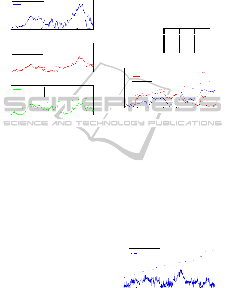
In figure 5 the estimation errors and the estimated
uncertainty regions for an exemplary trajectory are vi-
sualized. The uncertainty regions are defined by the
95% confidence interval. As can be seen the error for
the estimated position using PD bounds the true tra-
jectory error. In contrast the ID becomes inconsistent
with increasing time. The ES estimation is highly in-
consistent, even after a few estimations.
Using an average of 35 landmarks the average run-
time is 53.8[ms], 87.5[ms] and 69.8[ms] per estima-
tion for ES, ID and PD respectively. The tests were
carried out on a desktop pc (Intel(R) Core(TM) i7
@ 2.67GHz) using a interpreter simulation software
(MathWorks MatLab(R)) without exploiting sparse
matrix structures. That is, the computational effort
for all estimators can be reduced significantly by us-
ing efficient programming and sparse matrices.
6 EXPERIMENTS
In this section some experiments performed on the
dataset provided by the Rawseeds Project (see sec. 1)
are presented. The complete dataset includes 26000
images. For this evaluation only a subset is used con-
taining 14200 images and a traveled distance of 376
VISAPP 2012 - International Conference on Computer Vision Theory and Applications
150
200 400 600 800 1000
0
2
4
estimation step
ε
x
[bl]
200 400 600 800 1000
0
2
4
estimation step
ε
x
[bl]
200 400 600 800 1000
0
2
4
estimation step
ε
x
[bl]
ES pos. error
ES 2σ bound
ID pos. error
ID 2σ bound
PD pos. error
PD 2σ bound
Figure 5: Estimation error ε
x
for x-position in baselines and
2σ bounds for ES, ID and PD respectively.
meters. Ground truth information is available only for
the movement in the X/Z-plane and the systems head-
ing. Thus, only a 3 DOF pose is estimated here. In
addition to the pose parameters the systems velocity
is included in the estimation to model system motion.
Data provided by a low cost IMU is used for predict-
ing the velocity and orientation.
In contrast to section 5 only points with dispari-
ties ≤ 0 are rejected. If such disparities occur during
state updates, the respective point is excluded from
the state and the iteration process is continued. This
has proven to be a feasible exception handling and
during all tests the estimators convergence was not ef-
fected. Moreover, because the uncertainty of dispar-
ities rapidly decreases due to camera translation and
stereo constraints this has to be applied very seldom
(about 30 times for 14200 estimation steps).
For the global poses standard deviations the
square root of summed variances of the incremental
poses are used (see sec. 4.3). The absolute trajectory
errors and their estimated standard deviations are vi-
sualized in figures 6 and 7 respectively. Table 3 lists
the standard deviations and means of these errors. In
addition the tables first row shows the means of the
standard deviations estimated by the KF.
As can be seen the position and orientation esti-
mates are consistent with the estimated covariance.
Moreover the estimation is informative, that is, the
standard deviations are not estimated as too large.
Table 3: First and second row: means of standard devia-
tions for trajectory error in x- and z-position ε
x
,ε
z
in [m] and
heading ε
h
in [deg], estimated using our method and com-
puted empirically from trajectory error. Third row: mean of
absolute errors.
kε
x
k kε
z
k kε
h
k
estimated std. 0.56 0.75 1.65
empirical std. 0.52 0.48 0.74
mean abs. error 0.79 0.81 1.26
0 2000 4000 6000 8000 10000 12000 14000
0
0.5
1
1.5
2
2.5
3
3.5
4
abs. position error
frame number
meters
error X
3σ range
error Z
3σ range
Figure 6: Absolute position error and 3σ range without ad-
justment.
The trajectory starts with a heading of 0 (z-axis di-
rection) and no movement for some frames. Thus,
the uncertainty of the velocity only effects the posi-
tions z-component so its variance is higher than in
x-direction. The same effect can be observed at im-
age index 12000. Here the system stops in front of
a white wall, thus, no visual features are present for
some frames.
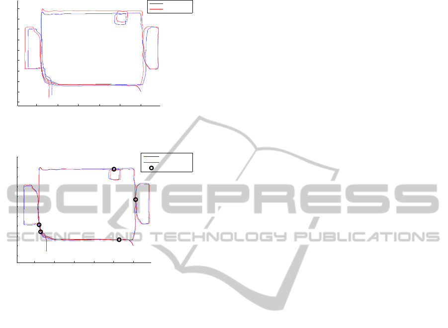
The global trajectory estimate is visualized in fig-
ure 8. The trajectory estimate shows the reliabil-
ity of pose estimation even without adjustment. This
proves, that an automatic detection of closed loops
could be applied by matching key frames for close-
by positions estimates. In figure 9 an adjusted esti-
mation is shown, using hand selected key points and
a constraint to poses only. That is, no bundle adjust-
ment was performed, but the poses increments inside
a loop are constrained to sum up to 0. Because the
0 2000 4000 6000 8000 10000 12000 14000
0
1
2
3
4
5
6
7
degrees
image number
abs. heading error
3σ range
Figure 7: Absolute heading error and 3σ range without ad-
justment.
A NOVEL STATE PARAMETRIZATION FOR STEREO-SLAM
151
−50 −40 −30 −20 −10 0
−5
0
5
10
15
20
25
30
35
40
position [m] before adjustment
estimated
ground truth
Figure 8: Estimated trajectory in [m] without adjustment.
−50 −40 −30 −20 −10 0
−5
0
5
10
15
20
25
30
35
40
45
position [m] after adjustment
estimated
ground truth
keyframe
Figure 9: Estimated trajectory in [m] after adjustment.
Black circles mark loop close positions.
velocity in the systems body frame was constraint to
be consistent with the position increment, the velocity
and heading were also improved.
For the used dataset the system performs at about
6-7 fps using a desktop PC with an average of 16.5
landmarks. Since the software is programmed using a
rapid prototyping framework including visualization
of landmarks and without optimizations this can be
improved. A great deal of time (about 30%) is spent
with the generation of KLT-features because a simple
CPU implementation is used. Moreover taking ad-
vantage of the sparse Jacobian matrices would speed
up the system. Keeping this in mind we are confident
that a frame rate of 20 to 30 fps can be achieved.
The system models are applicable to full 6 DOF
pose estimation also, as introduced in chapter 4. Ex-
periments on the same dataset apparently yield good
results. Especially the height (Y-axis) was estimated
reliably. The final deviation for the complete trajec-
tory was about 2 to 3 meters (close to 1% of trajectory
length), assuming start and end point have the same
height. This is notable, since IMUs are known to be
highly unstable predicting the height (parallel to grav-
ity acceleration). Since ground truth information is
given for 3 DOF only, these results are not discussed
further here.
7 CONCLUSIONS
We have introduced a novel parametrization for stereo
SLAM systems. Because of optimal exploitation of
stereo constraints the observation models are nearly
linear and the parametrization is minimal. Moreover
it meets the assumption of Gaussian noise, such that
it is predestinated for application in linear estimators
like kalman filters.
It was proven in synthetical tests and real-world
experiments, that the estimation is precise and con-
sistent even for long term estimation. The synthetical
tests showed that for stereo systems the PD outper-
forms the ID in terms of computational effort and co-
variance estimation, i.e. the consistency is preserved.
Consistent variance estimation is a major advance-
ment for navigation, since it improves long term sta-
bility, reliability information and the quality of global
adjustments. Moreover, due to the reduction in com-
putational costs for PD, much more landmarks can be
used to improve the estimations accuracy. The exper-
iments using the RawSeed data showed the applica-
bility of the proposed methods to actual SLAM prob-
lems.
For future work it is planed to introduce points at
infinity as was done for ID. These are characterized by
a disparity equal to 0. Thus, they can be modeled us-
ing the same observation model (see equation 10) and
parametrization, by omitting the disparity component
(fixed to 0). This way the points, rejected due to pos-
sibly negative disparities, can be exploited to improve
orientation estimation. Another task is to generalize
the modeling to monocular SLAM systems, for exam-
ple by using epipolar lines for offset (disparity) repre-
sentation.
REFERENCES
Bonarini, A., Burgard, W., Fontana, G., Matteucci, M., Sor-
renti, D. G., and Tardos, J. D. (2006). Rawseeds:
Robotics advancement through web-publishing of
sensorial and elaborated extensive data sets. In pro-
ceedings of IROS’06 Workshop on Benchmarks in
Robotics Research.
Brooks, R. (1985). Visual map making for a mobile
robot. In Proceedings IEEE International Conference
on Robotics and Automation 1985, volume 2, pages
824 – 829.
Ceriani, S., Fontana, G., Giusti, A., Marzorati, D., Mat-
teucci, M., Migliore, D., Rizzi, D., Sorrenti, D. G.,
and Taddei, P. (2009). Rawseeds ground truth collec-
tion systems for indoor self-localization and mapping.
Autonomous Robots, 27(4):353–371.
Civera, J., Davison, A. J., and Montiel, J. M. M. (2008). In-
VISAPP 2012 - International Conference on Computer Vision Theory and Applications
152

verse depth parametrization for monocular slam. Au-
tonomous Robots, 24(5):932–945.
Crowley, J. L. (1989). World modeling and position esti-
mation for a mobile robot using ultrasonic ranging. In
IEEE Conference on Robotics and Automation, pages
1574–1579.
Dissanayake, M. W. M. G., Newman, P., Clark, S., Durrant-
Whyte, H. F., and Csorba, M. (2001). A solution to
the simultaneous localization and map building (slam)
problem. Transactions on Robotics and Automation,
17(3):229–241.
Hartley, R. and Zisserman, A. (2003). Multiple View Geom-
etry. Cambirdge University Press, 2 edition.
Herath, D. C., Kodagoda, K. R. S., and Dissanayake, G.
(2006). Modeling errors in small baseline stereo for
slam. Technical report, ARC Centre of Excellence in
Autonomous Systems (CAS).
Hildebrandt, M. and Kirchner, F. (2010). Imu-aided stereo
visual odometry for ground-tracking auv applications.
Technical report, Underwater Robotics Department,
DFKI RIC Bremen.
˙
Imre, E. and Berger, M.-O. (2009). A 3-component inverse
depth parameterization for particle filter slam. In Lec-
ture Notes in Computer Science, volume 5748/2009,
pages 1–10. Springer.
Kalman, R. E. (1960). A new approach to linear filtering
and prediction problems. Journal of Basic Engineer-
ing, 82.
Lefebvre, T., Bruyninckx, H., and De Schutter, J. (2004).
Kalman filters for non-linear systems: a comparison
of performance. International Journal of Control,
77(7).
Lemaire, T., Berger, C., Jung, I.-K., and Lacroix, S. (2007).
Vision-based slam: Stereo and monocular approaches.
International Journal of Computer Vision, 73(3):343–
364.
Leonard, J. and Durrant-Whyte, H. (1992). Directed Sonar
Sensing for Mobile Robot Navigation. Springer.
McGlone, J. C., F
¨
orstner, W., and Wrobel, B. (2004). Man-
ual of Photogrammetry, chapter 2 Mathematical Con-
cepts in Photogrammetry. asprs.
Paz, L. M., Pini
´
es, P., Tard
´
os, J. D., and Neira, J. (2008).
Large-scale 6-dof slam with stereo-in-hand. Transac-
tions on Robotics, 24(5).
Petersen, A. and Koch, R. (2010). Statistical analysis of
kalman filters by conversion to gauss-helmert models
with applications to process-noise estimation. In Pro-
ceedings of ICPR2010, Istanbul, Turkey.
Schleicher, D., Bergasa, L. M., Barea, R., L
´
opez, E., Ocana,
M., Nuevo, J., and Fern
´
andez, P. (2007). Real-time
stereo visual slam in large-scale environments based
on sift fingerprints. Technical report, Department of
Electronics, University of Alcal
´
a.
Sol
´
a, J., Monin, A., and Devy, M. (2007). Bicamslam: Two
times mono is more than stereo. In Proceedings of
IEEE International Conference on Robotics and Au-
tomation, pages 4795–4800, Rome, Italy.
Song, Y., Song, Y., and Li, Q. (2011). Robust iterated sigma
point fastslam algorithm for mobile robot simultane-
ous localization and mapping. Chinese Journal of Me-
chanical Engineering, 24.
S
¨
underhauf, N., Lange, S., and Protzel, P. (2007). Using
the unscented kalman filter in mono-slam with inverse
depth parametrization for autonomous airship control.
In Proceedings of IEEE International Workshop on
Safety Security and Rescue Robotics.
Uhlmann, J. K. (2003). Covariance consistency methods
for fault-tolerant distributed data fusion. Information
Fusion, 4(3):201 – 215.
Welch, G. and Bishop, G. (2006). An introduction to the
kalman filter. Technical report, University of North
Carolina at Chapel Hill, Chapel Hill, NC, USA.
A NOVEL STATE PARAMETRIZATION FOR STEREO-SLAM
153
