IMPROVING RAY TRAVERSAL BY USING SEVERAL
SPECIALIZED KD-TREES
Roberto Torres, Pedro J. Mart
´
ın, Antonio Gavilanes and Luis F. Ayuso
Departamento de Sistemas Inform
´
aticos y Computaci
´
on, Universidad Complutense de Madrid, Madrid, Spain
Keywords:
Ray Tracing, Surface Area Heuristics, KD-tree, GPU, CUDA.
Abstract:
In this paper, we present several variants of the Surface Area Heuristics (SAH) to build kd-trees for specific
sets of rays’ directions. In order to cover the whole space of directions, several sets of directions are considered
and each of them leads to a different specialized kd-tree. We call Multi-kd-tree to the set of these kd-trees.
During rendering, each ray will traverse the kd-tree associated with the set containing its direction. In order
to evaluate the efficiency of our proposal, we have implemented a Path Tracing and an Ambient Occlusion
renderer on GPU with CUDA. A SAH-based kd-tree has been compared to a Multi-kd-tree and we show that
all the new heuristics exhibit a better performance than SAH over usual scenes.
1 INTRODUCTION
Ray tracing algorithms cover a family of algorithms
devoted to the generation of 2D images from a 3D
representation of the scene. In these algorithms, ren-
dering is carried out by shooting rays throughout the
scene. The final results usually exceed in realism
those obtained with the graphics pipeline algorithm.
This is the reason why ray tracing is the favourite
choice in the generation of photo-realistic images
(Pharr and Humphreys, 2010).
A common task of every ray tracer, which is usu-
ally the most time-consuming step, is to find the near-
est intersection per ray (traversal step). In order to ac-
celerate this task, several data structures have been de-
veloped to organize the scene. Their advantage is that
their traversal algorithms can quickly reject whole re-
gions, avoiding many intersection tests. Examples of
these structures are uniform grids, kd-trees, octrees
and bounding volume hierarchies (BVHs).
The most efficient hierarchical structures for ray
tracing are built with SAH (Goldsmith and Salmon,
1987) using the greedy top-down algorithm by (Mac-
Donald and Booth, 1990), originally presented for kd-
trees, and later adapted to BVHs by (Wald, 2007).
However, SAH involves assumptions about rays than
can be replaced by more realistic ones to build
structures with better performance during rendering
(Havran and Bittner, 1999; Hunt and Mark, 2008;
Fabianowski et al., 2009; Bittner and Havran, 2009).
On the other hand, GPUs are massively-parallel
devices that have been used to implement ray tracers,
typically binding each thread to a ray during traver-
sal. However, a thread can stall others in the under-
lying SIMT architecture, mainly due to global mem-
ory readings and runtime divergences. This fact has
led the design of effective GPU-based ray traversal.
The first proposals (G
¨
unther et al., 2007; Popov et al.,
2007), which were based on ray packets as traversal
units, were discarded by (Aila and Laine, 2009) be-
cause many rays were forced to traverse regions of
the scene they did not intersect. Nevertheless, an ap-
propriate arrangement of rays in the device can ex-
ploit coalesced readings and cache hits of modern
hardware. Therefore, recent trends use data-parallel
primitives to rearrange rays in the device either at the
beginning (Garanzha and Loop, 2010) or repeatedly
during the traversal (Torres et al., 2011). The aim is
to get a trade-off between the overload due to the re-
arrangement of rays and the increase of performance.
The main contribution of this paper is the develop-
ment of new heuristics from a mathematical formula-
tion of the original SAH. These heuristics specialize
SAH for different sets of ray directions by restrict-
ing their domain or by assuming non-uniform prob-
abilities. In order to cover the whole space of di-
rections, several sets are used and a kd-tree is built
for each of them. The set of these kd-trees is called
a Multi-kd-tree. We have tested our heuristics using
two ray tracing algorithms implemented with CUDA:
Path Tracing and Ambient Occlusion. Before travers-
ing, secondary rays are classified and arranged on the
215
Torres R., J. Martín P., Gavilanes A. and F. Ayuso L..
IMPROVING RAY TRAVERSAL BY USING SEVERAL SPECIALIZED KD-TREES.
DOI: 10.5220/0003844702150226
In Proceedings of the International Conference on Computer Graphics Theory and Applications (GRAPP-2012), pages 215-226
ISBN: 978-989-8565-02-0
Copyright
c
 2012 SCITEPRESS (Science and Technology Publications, Lda.)

device according to the Multi-kd-tree components.
In both renderers, Multi-kd-trees exhibit better be-
haviour than a single SAH-based kd-tree over usual
scenes, concerning traversal steps and runtime perfor-
mance.
2 RELATED WORK
There is an extensive literature about acceleration
structures for ray tracing. (Havran, 2000) proved that
SAH-based kd-trees were very efficient concerning
static scenes on CPU. Thus, subsequent work tried
to move these structures from CPU to GPU. (Foley
and Sugerman, 2005) presented two techniques to tra-
verse kd-trees without a stack: kd-tree restart and kd-
tree backtrack. Nevertheless, the amount of traversed
nodes was greater than the one involved in the classic
traversal, due to the fact that many nodes were visited
several times. (Horn et al., 2007) improved kd-tree
restart by using a small fixed-size stack taking ad-
vantage of the new GPU characteristics. In addition,
(Popov et al., 2007) implemented a kd-tree traversal
without stack on GPU by using ropes and ray packets.
As far as BVHs are concerned, (Thrane et al.,
2005) was the first proposal in implementing a BVH
on GPU. Afterwards, (G
¨
unther et al., 2007) designed
a packet-based BVH traversal on CUDA by means
of a stack that was implemented on shared memory.
(Torres et al., 2009) implemented a stackless traver-
sal on a roped BVH using packets. After that, (Aila
and Laine, 2009) proved that a single-ray traversal on
BVH is faster than a packet-based one due to the high
memory bandwidth of GPUs. (Garanzha and Loop,
2010) developed a faster traversal by sorting the rays
and breath-first traversing the BVH.
Regarding SAH, several papers have focused on
improving it for specific sets of rays. (Havran and Bit-
tner, 1999) presented several heuristics where proba-
bilities are approximated as ratios of areas by using
either orthogonal, perspective or spherical projection.
Recently, (Hunt and Mark, 2008) developed a new
heuristics adapted to rays in perspective space to build
kd-trees by using oblique projections. (Fabianowski
et al., 2009) designed a variant of SAH supposing that
rays’ origins are inside the scene, which is suitable
for secondary and shadow rays. (Bittner and Havran,
2009) used a representative ray set to approximate the
probability as the ratio of the number of intersected
rays.
3 KD-TREE BASED ON SAH
A kd-tree is a binary tree responsible for organizing
the objects in the scene. The volume associated with
the root is the AABB (Axis-Aligned Bounding Box)
of the whole scene and each inner node contains a
plane aligned with the axes that subdivides this vol-
ume into two voxels. Thus, the volume associated
with each node is the AABB that results from reduc-
ing the root’s voxel with its ancestor planes. In addi-
tion, each leaf contains a list of triangles overlapping
its AABB.
In order to build good kd-trees, it is essential to
measure their quality. This is usually formalized by
the following recursive cost function (MacDonald and
Booth, 1990):
Cost(l) = Cost
tri
· N
tri
(l)
Cost(i) = Cost
plane
+ P(L|i) ·Cost(L)
+ P(R|i) ·Cost(R)
where l is a leaf node, i is an inner node, L and R
respectively denote the left and right children of i,
Cost
tri
is the cost of intersecting a ray with a triangle,
N
tri
(l) is the number of triangles of l, and Cost
plane
is
the cost of intersecting a ray with a plane. P(A|B) is
the probability for any ray to intersect the AABB of
node A, provided that it already intersects the AABB
of node B.
The aim of the construction is to find a kd-tree
with minimum cost. However, there are two values in
the previous equations that have to be estimated: the
probability P(·|·) and the costs related to the children
L and R.
With respect to the children’s costs, trying to build
all possible trees and choosing the one minimizing the
cost is unfeasible in general. Therefore, children are
assumed to be leaves and so, their costs are quickly
computed according to the cost function. In con-
sequence, the construction behaves as a greedy top-
down algorithm that looks for the best division of an
inner node into two new leaves with the lowest local
cost. We follow the O(NlogN) algorithm by (Wald
and Havran, 2006) for the kd-tree construction.
The probability P(A) can be evaluated by using
geometric probability as a ratio of measures
P(A) =
µ(A)
µ(Scene)
where A is the AABB of a node and Scene is the
AABB of the whole scene —for the sake of clarity,
we will identify a node with its AABB along this pa-
per. Notice that, if A and B are AABBs inside Scene
and A ⊆ B, then
P(A|B) =
P(A∩ B)
P(B)
=
P(A)
P(B)
=
µ(A)
µ(B)
GRAPP 2012 - International Conference on Computer Graphics Theory and Applications
216

In order to specify µ, three facts are usually
assumed about rays’ directions (Wald and Havran,
2006):
1. All directions are equally likely, i.e. they have
constant probability.
2. The origin of each ray is out of the scene.
3. The rays do not get blocked during the traversal,
i.e. they finish out of the scene.
Notice that these assumptions consider directions as
lines, i.e. directions ω and −ω result in the same
line. So, one half of the vectors on the unit sphere
are enough to cover all rays.
A particular measure µ
1
leads to the original SAH
formulation as follows. Consider the function hit
r
(A)
that returns 1 when a ray r hits the AABB A, and 0
otherwise. Under the previous assumptions, hit
r
(A)
can be estimated as the projected area of A on any
plane whose normal is the direction ω of the ray r.
Thus, if we consider a set of rays, the measure is the
integral over the domain of directions. As explained
above, a hemisphere H on the unit sphere is enough
to cover all directions. Mathematically, the measure
µ
1
is then expressed as
µ
1
(A) =
Z
ω∈H
proj orth(A,ω) dσ(ω)
where ω is a unit ray direction, dσ is the differential
solid angle and proj orth(A,ω) is the area of the or-
thogonal projection of A on any plane whose normal
is ω.
Since we work with AABBs, the latter measure
can be evaluated as follows, using the hemisphere
with ω
Z
≥ 0:
µ
1
(A) =
Z
ω∈H
∑
i∈{X,Y,Z}
|N
i
· ω|A
i
dσ(ω)
=
Z
π
2
0
Z
2π
0
(|ω
X
| · A
X
+ |ω
Y
| · A
Y
+ |ω
Z
| · A
Z
)sinθ dφdθ
= 2π(A
X
+ A
Y
+ A
Z
)
where A
X
, A
Y
and A
Z
are the areas of one face of each
pair of parallel faces, and N
X
= (1,0,0), N
Y
= (0,1,0)
and N
Z
= (0,0, 1) are their normals. If SA(A) de-
notes the surface area of the AABB A, the probability
P(A|B) can be computed as
P(A|B) =
µ
1
(A)
µ
1
(B)
=
2π(A
X
+ A
Y
+ A
Z
)
2π(B
X
+ B
Y
+ B
Z
)
=
SA(A)
SA(B)
which corresponds to the SAH formulation.
θ
φ
x
y
z
x
y
z
1
Figure 1: Distribution of the spherical patches (left) and cu-
bic patches (right). For the sake of clarity, the six patches
are shown in both figures, however, only three are consid-
ered.
4 SPECIALIZED HEURISTICS
The original SAH assumes three facts about rays
(Section 3). We will define variants of SAH by chang-
ing the original assumptions about rays’ directions:
1. Considering different sets of directions rather than
the whole hemisphere. This leads to specialized
kd-trees that result in better performance for rays
whose directions belong to these sets.
2. Considering a non-uniform distribution for rays.
Given a direction N, we will suppose that rays
are more probable as their directions are closer
to N. This results in a kd-tree specialized in the
surroundings of N.
In addition, we generalize the way hit
r
(A) is es-
timated using oblique projections. Actually, we will
consider orthogonal and oblique projections under the
two new assumptions.
4.1 Spherical Heuristics
We relax the assumption that every ray is possible by
restricting the directions to a fixed set. Nevertheless,
we keep on assuming that the probability of all rays
is uniform. Specifically, we split half of the direction
space into three pairwise disjoint spherical patches as
Figure 1 on the left shows. In that sense, the three
spherical patches can be expressed as
SP
i
=
{
(sinθcosφ, sinθsinφ, cosθ) | θ ∈ Θ
i
,φ ∈ Φ
i
}
where i ∈ {X,Y,Z}, and Θ
i
and Φ
i
are the intervals in
Table 1. The value θ
0
= acos(
2
3
) has been chosen for
the patches to have the same area and, therefore, the
sets of directions have the same size.
As mentioned, we have two possibilities for
choosing the projection. Thereby, SPHERE-ORTH
and SPHERE-OBLI will respectively denote the
heuristics for the orthogonal and oblique projection.
IMPROVING RAY TRAVERSAL BY USING SEVERAL SPECIALIZED KD-TREES
217

Table 1: Bounds and normalized weights for spherical and cubic heuristics. The values w
X
, w
Y
and w
Z
are the normalized
weights in percentage for the face areas A
X
, A
Y
and A
Z
, respectively.
Patch Bounds (spherical coord.) SPHERE-ORTH SPHERE-OBLI
Θ Φ w
X
w
Y
w
Z
w
X
w
Y
w
Z
SP
X
[θ
0
,π− θ
0
] [
−π
4
,
π
4
] 55.04 22.80 22.15 53.47 23.59 22.92
SP
Y
[θ
0
,π− θ
0
] [
π
4
,
3π
4
] 22.80 55.04 22.15 23.59 53.47 22.92
SP
Z
[0,θ
0
] [0,2π] 22.04 22.04 55.90 22.66 22.66 54.67
Patch Bounds (cartesian coord.) CUBE-ORTH CUBE-OBLI
x y z w
X
w
Y
w
Z
w
X
w
Y
w
Z
CP
X
{1} [−1,1] [−1,1] 51.29 24.35 24.35 50.00 25.00 25.00
CP
Y
[−1,1] {1} [−1,1] 24.35 51.29 24.35 25.00 50.00 25.00
CP
Z
[−1,1] [−1,1] {1} 24.35 24.35 51.29 25.00 25.00 50.00
In that way, each spherical patch represents a set
of directions and leads to one different measure per
projection type. The three measures for SPHERE-
ORTH are
µ
(i)
2
(A) =
Z
ω∈SP
i
proj orth(A,ω) dσ(ω)
for the patches SP
i
, i ∈ {X,Y,Z}. For example, the
probability P(A|B) for patch SP
X
in SPHERE-ORTH
is
P(A|B) =
µ
(X)
2
(A)
µ
(X)
2
(B)
=
w
X
· A
X
+ w
Y
· A
Y
+ w
Z
· A
Z
w
X
· B
X
+ w
Y
· B
Y
+ w
Z
· B
Z
=
0.5504· A
X
+ 0.2280· A
Y
+ 0.2215· A
Z
0.5504· B
X
+ 0.2280· B
Y
+ 0.2215· B
Z
In general, when the integrals are solved, we ob-
tain a weighted addition of the areas A
X
, A
Y
and A
Z
.
After that, we normalize these values by extracting
their sum as a common factor. We call these nor-
malized weights w
X
, w
Y
and w
Z
, whose values have
been included for the three spherical patches in Ta-
ble 1. Notice how the area A
X
has a bigger weight
when considering rays with directions on the spheri-
cal patch SP
X
. The use of SPHERE-ORTH leads to
three different kd-trees, one for each spherical patch,
i.e. the measure µ
(i)
2
is used during the construction of
the kd-tree related to SP
i
.
In SPHERE-OBLI, the planes for the oblique pro-
jection must be chosen. We have tested the planes YZ
for SP
X
, XZ for SP
Y
and XY for SP
Z
. E.g., the mea-
sure for SP
Z
is
µ
(Z)
3
(A) =
Z
ω∈SP
Z
proj obli
XY
(A,ω) dσ(ω)
=
Z
ω∈SP
Z




ω
X
ω
Z




A
X
+




ω
Y
ω
Z




A
Y
+ A
Z
dσ(ω)
By solving the integrals and normalizing the weights,
we obtain
P(A|B) =
0.2266· A
X
+ 0.2266· A
Y
+ 0.5467· A
Z
0.2266· B
X
+ 0.2266· B
Y
+ 0.5467· B
Z
for SP
Z
. See Table 1 for the normalized weights re-
lated to SP
X
and SP
Y
.
4.2 Cubic Heuristics
Other sets of directions can be obtained if they are
taken on the surface of a cube. Similar to (Hunt and
Mark, 2008), we have chosen the cube [−1,1]
3
as Fig-
ure 1 shows on the right. As before, directions are
considered as lines, so we use three faces on the cube.
They are pairwise disjoint and called cubic patches
CP
X
, CP
Y
and CP
Z
. We call CUBE-ORTH to the
heuristics when the orthogonal projection is used, and
CUBE-OBLI if the oblique projection is applied.
The new three measures in CUBE-ORTH are
µ
(i)
4
(A) =
Z
ω∈CP
i
proj orth

A,
ω
|ω|

dA(ω)
for i ∈ {X,Y,Z}. Notice the normalization of the vec-
tor ω unlike the spherical heuristics. For example, the
measure for CP
Z
is
µ
(Z)
4
(A) =
Z
1
−1
Z
1
−1
proj orth A,
(x,y,1)
p
x
2
+ y
2
+ 1
!
dxdy
By solving and normalizing, the probability for CP
Z
is
P(A|B) =
0.2435· A
X
+ 0.2435· A
Y
+ 0.5129· A
Z
0.2435· B
X
+ 0.2435· B
Y
+ 0.5129· B
Z
In CUBE-OBLI, the oblique projection is taken
into account. Using the same projection planes used
for SPHERE-OBLI, we obtain the measure for CP
Z
as
follows
µ
(Z)
5
(A) =
Z
ω∈CP
Z
proj obli
XY

A,
ω
|ω|

dA(ω)
=
Z
1
−1
Z
1
−1
|x| · A
X
+ |y| · A
Y
+ A
Z
dxdy
= 4
Z
1
0
Z
1
0
x· A
X
+ y· A
Y
+ A
Z
dxdy
GRAPP 2012 - International Conference on Computer Graphics Theory and Applications
218

Table 2: Normalized weights in percentage for cosine
heuristics, taking different values of β. We only present the
case for N
X
. The other cases can be obtained by suitably
swapping columns.
COS-ORTH COS-OBLI
β w
X
w
Y
w
Z
w
X
w
Y
w
Z
1 43.99 28.00 28.00 33.33 33.33 33.33
2 50.00 25.00 25.00 43.99 28.00 28.00
3 54.08 22.95 22.95 50.00 25.00 25.00
4 57.14 21.42 21.42 54.08 22.95 22.95
5 59.55 20.22 20.22 57.14 21.42 21.42
10 67.01 16.49 16.49 65.90 17.04 17.04
Then
P(A|B) =
0.25· A
X
+ 0.25· A
Y
+ 0.5· A
Z
0.25· B
X
+ 0.25· B
Y
+ 0.5· B
Z
for CP
Z
. Similar expressions can be obtained for CP
X
and CP
Y
. Table 1 displays the values of the normal-
ized weights for these heuristics.
4.3 Cosine Heuristics
In this heuristics, we assume that all directions are
possible but all of them are not equally probable. We
will suppose that directions near a given unit direc-
tion N are more likely than others. We accomplish it
by multiplying the projected area related to a unit di-
rection ω by the factor (ω· N)
β
, where β is a positive
real number. Again, two types of projections can be
considered, resulting in two heuristics, COS-ORTH
for orthogonal projections and COS-OBLI for oblique
projections.
We have tested three values for the direction N,
N
X
= (1,0,0), N
Y
= (0,1,0) and N
Z
= (0,0,1). For
each of them we have integrated over the hemisphere
surrounding N, that is, we have used the hemispheres
with ω
X
≥ 0, ω
Y
≥ 0 and ω
Z
≥ 0, denoted as H
X
,
H
Y
and H
Z
, respectively. Each hemisphere leads to a
different measure and it produces a specific kd-tree.
Notice that domains are not pairwise disjoint for the
cosine heuristics.
The measures for COS-ORTH and COS-OBLI are
respectively
µ
(i)
6
(A) =
Z
ω∈H
i
(ω· N
i
)
β
· proj orth(A,ω) dσ(ω)
µ
(i)
7
(A) =
Z
ω∈H
i
(ω· N
i
)
β
· proj obli(A,ω) dσ(ω)
for i = {X,Y,Z}. In Table 2, we present the nor-
malized weights for N
X
, taking different values of β.
The weights for N
Y
and N
Z
result from permuting the
weights for N
X
, since one rotation of π/2 radians is
enough to transform H
X
into H
Y
or H
Z
.
5 KD-TREE SELECTION
We apply the O(NlogN) top-down algorithm by
(Wald and Havran, 2006) for the kd-tree construction.
However, instead of using the surface area to calcu-
late the conditional probability, we apply any of the
measures above described. We call kd-tree
(i)
n
to the
kd-tree built with µ
(i)
n
(the n-th measure and the set
of directions SP
i
or CP
i
, or the normal N
i
). Since,
the use of a single kd-tree for the whole scene would
benefit some rays but would penalize others, we build
three kd-trees (kd-tree
(X)
n
, kd-tree
(Y)
n
and kd-tree
(Z)
n
)
in order to cover the whole direction space. We call
Multi-kd-tree to the set of these kd-trees.
The process of traversing a Multi-kd-tree by a ray
in the spherical and cubic heuristics can be summa-
rized as follows. First of all, each ray selects the
kd-tree to traverse. In the case of cubic patches,
it is identical to the selection of a face in the cube
mapping technique. In the case of spherical patches,
if |ω
Z
| > cos(θ
0
) then the ray chooses kd-tree
(Z)
n
,
and otherwise max(|ω
X
|,|ω
Y
|) is used to choose kd-
tree
(X)
n
or kd-tree
(Y)
n
. Once a kd-tree of the Multi-kd-
tree is selected by the ray, it is subsequently traversed
as usual.
For the cosine heuristics, we use the kd-trees re-
lated to normals N
X
, N
Y
and N
Z
. Each ray chooses the
kd-tree to traverse by using the selection procedure of
the spherical heuristics.
6 IMPLEMENTATION DETAILS
We have implemented a Path Tracing (PT) and
an Ambient Occlusion (AO) on CUDA to test the
performance of a Multi-kd-tree according to the
new heuristics. The scenes used in our tests are
BUNNY, FAIRYFOREST, CONFROOM, SPONZA and
SIBENIK (Tables 6 and 7). A roof has been added
to FAIRYFOREST and a bounding box enclosing
BUNNY to prevent the rays from getting away from
the scene. The images generated have a resolution of
1024× 1024 and every surface is diffuse.
The construction of all kd-trees is made on CPU
before rendering. The time spent in the construction
of each kd-tree with the new heuristics is almost the
same as with SAH.
Before rendering, all the kd-trees needed are allo-
cated together on device memory. In the node array,
all the nodes of these kd-trees are allocated, and the
nodes corresponding to the same kd-tree are contigu-
ous. In the reference array, the references to triangles
of every leaf are stored. The indices to the root of
IMPROVING RAY TRAVERSAL BY USING SEVERAL SPECIALIZED KD-TREES
219

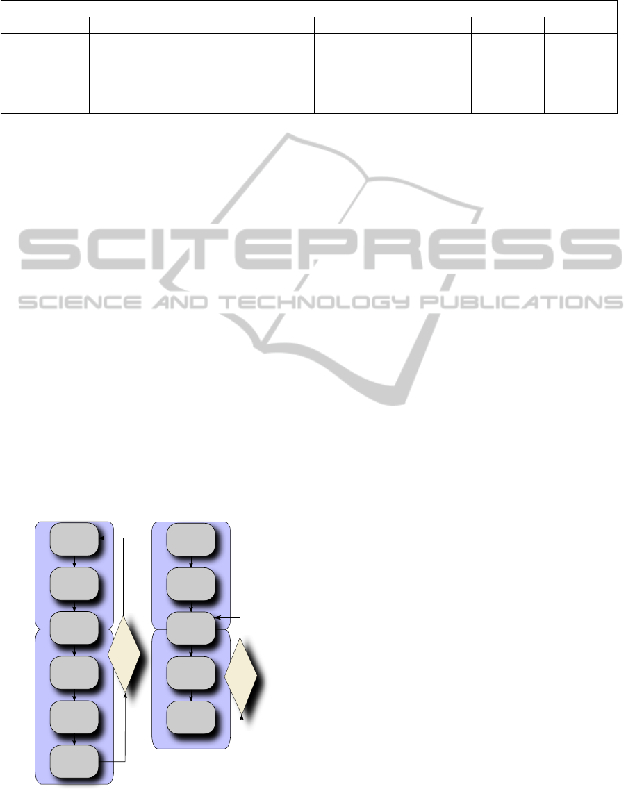
Table 3: Number of triangles and memory footprint used by a SAH-based kd-tree and a Multi-kd-tree built with SPHERE-
ORTH. Num.Nodes is the number of nodes (either inner or leaf) of the kd-trees. Num.Ref. is the total number of references to
triangles inside the leaves. Each node requires 16 bytes and each reference 4 bytes.
SAH SPHERE-ORTH
Scene Triangles Num.Nodes Num.Ref. Memory Num.Nodes Num.Ref. Memory
BUNNY 69,475 536,639 343,082 9.49 MB 1,738,331 1,092,768 30.69 MB
F.FOREST 174,119 1,257,457 922,883 22.70 MB 3,983,961 2,901,640 71.85 MB
CONFROOM 282,761 1,570,225 1,433,336 29.42 MB 5,253,325 4,723,711 98.17 MB
SPONZA 67,464 436,899 367,534 8.06 MB 1,339,641 1,141,669 24.79 MB
SIBENIK 80,143 358,779 311,503 6.66 MB 1,100,537 965,394 20.47 MB
each kd-tree are stored on another array, the header
array. Table 3 shows the number of nodes (either
inners or leaves) and the memory footprint used by
a SAH-based kd-tree and a Multi-kd-tree built with
SPHERE-ORTH. As it can be seen, the used mem-
ory of the Multi-kd-tree is about three times the space
required by a SAH-based kd-tree. The remaining
heuristics exhibit similar memory requirements.
Path Tracing. This renderer considers two lev-
els of recursion: primary rays and secondary rays. It
is composed of three kernels: RayGeneration (RG),
TraversalIntersection (TI) and Shading (SH). The
flowchart of the CUDA kernels can be seen in Figure
2 on the left. Notice that this algorithm is an implicit
path tracer, i.e. no shadow ray is traced from the in-
tersection points to lights. In order to complete the
final image, several iterations of the kernels are used,
being its number externally controlled.
Kernel RG is devoted to generating primary rays
from the camera (a pinhole camera). In each itera-
tion, four different random samples per pixel are gen-
erated, so the total amount of rays traced in parallel
Secondary Rays
Max.
Iterations?
RG
TI
SH
Sort
TI
SH
Primary Rays
Shadow Rays
Max.
Iterations?
RG
TI
SH
Sort
TI
Primary Rays
Figure 2: Flowchart of the kernels of Path Tracing (on the
left) and Ambient Occlusion (on the right).
is 4MRays = 4× 1024
2
rays per iteration. In this ker-
nel, each ray chooses the kd-tree to traverse as already
described (Section 5).
Kernel TI finds the nearest intersection point for
each ray. This kernel is actually the algorithm persis-
tent while-while by (Aila and Laine, 2009) adapted to
kd-trees. At the beginning of this kernel, the header
array is queried by each ray and the root of the kd-tree
is retrieved to start traversing.
Kernel SH accumulates the color of the rays in the
image buffer. If the rays are primary, then this ker-
nel also generates the new secondary ray from each
primary ray. These rays are generated on the hemi-
sphere surface according to the cosine probability. In
this kernel, and similar to RG, the new secondary rays
choose the kd-tree to be traversed on the subsequent
TI launching.
Ambient Occlusion. This renderer also consid-
ers two levels of recursion: primary rays and shadow
rays. It is also composed of three kernels (Figure 2 on
the right), which are very similar to the kernels of PT:
RayGeneration (RG), TraversalIntersection (TI) and
Shading (SH). In order to complete the final image,
multiple iterations of the shadow rays are executed, so
primary rays are only traced once at the beginning of
the render. In addition, RG only generates one sample
per pixel, so 1024
2
= 1MRays primary rays will be
traversed in parallel. In this kernel, identically to PT,
each ray selects the kd-tree to traverse.
TI has two configurations. In the first one, the
kernel finds the nearest intersection point for each ray,
which is suitable for primary rays. In the other, the
traversal is finished as soon as an intersection point is
found, which is suitable for shadow rays.
SH generates six shadow rays from each inter-
section point found by kernel TI. So 6 × 1024
2
=
6MRays shadow rays will be traversed in parallel in
each iteration. Each shadow ray chooses the kd-tree
to be traversed, similarly to primary rays.
Ray Arrangement. Primary rays are stored on an
array following the Morton code of the image pixels.
In this way, contiguous rays are very likely to choose
the same kd-tree to traverse. However, secondary rays
GRAPP 2012 - International Conference on Computer Graphics Theory and Applications
220

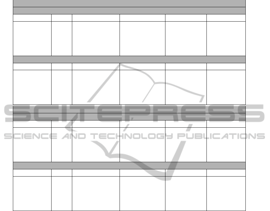
Table 4: Traversal Steps on average for Path Tracing and Ambient Occlusion. The number in parenthesis is the gain in
percentage w.r.t. SAH. Bold numbers are the maximum of each row.
Path Tracing
Primary Rays
Scene SAH SPHERE-ORTH SPHERE-OBLI CUBE-ORTH CUBE-OBLI
BUNNY 34.04 30.27(11.08) 32.30(5.11) 32.38(4.90) 32.33(5.02)
F.FOREST 48.82 45.38(7.04) 45.42(6.96) 45.70(6.38) 45.71(6.38)
CONFROOM 38.46 35.07(8.80) 34.78(9.56) 34.89(9.29) 35.01(8.96)
SPONZA 37.66 34.52(8.33) 34.74(7.75) 34.67(7.95) 34.97(7.13)
SIBENIK 45.03 39.39(12.51) 39.01(13.35) 38.43(14.63) 38.67(14.11)
Secondary Rays
Scene SAH SPHERE-ORTH SPHERE-OBLI CUBE-ORTH CUBE-OBLI
BUNNY 32.09 29.85(6.99) 30.88(3.78) 30.76(4.15) 30.75(4.18)
F.FOREST 51.51 48.71(5.43) 48.76(5.32) 49.11(4.65) 49.11(4.64)
CONFROOM 39.83 38.79(2.60) 38.83(2.50) 38.81(2.55) 38.77(2.66)
SPONZA 41.17 39.60(3.81) 39.53(3.98) 39.51(4.02) 39.50(4.06)
SIBENIK 48.01 46.01(4.16) 45.97(4.23) 46.02(4.13) 45.78(4.63)
Ambient Occlusion
Primary Rays
Scene SAH SPHERE-ORTH SPHERE-OBLI CUBE-ORTH CUBE-OBLI
BUNNY 34.23 30.46(10.99) 32.50(5.04) 32.57(4.83) 32.53(4.96)
F.FOREST 49.03 45.60(6.99) 45.64(6.90) 45.92(6.33) 45.92(6.33)
CONFROOM 38.55 35.17(8.76) 34.88(9.52) 34.98(9.26) 35.11(8.93)
SPONZA 37.73 34.59(8.31) 34.81(7.73) 34.74(7.93) 35.04(7.12)
SIBENIK 47.31 41.52(12.24) 41.13(13.06) 40.56(14.26) 40.80(13.75)
Shadow Rays
Scene SAH SPHERE-ORTH SPHERE-OBLI CUBE-ORTH CUBE-OBLI
BUNNY 28.91 26.44(8.55) 28.07(2.90) 28.19(2.50) 28.19(2.49)
F.FOREST 42.58 40.24(5.49) 40.29(5.36) 40.62(4.59) 40.65(4.52)
CONFROOM 31.28 30.84(1.41) 30.82(1.46) 30.77(1.63) 30.73(1.74)
SPONZA 34.35 33.02(3.86) 32.96(4.03) 32.96(4.03) 32.90(4.20)
SIBENIK 39.55 37.93(4.10) 37.89(4.20) 37.94(4.06) 37.82(4.36)
are randomly generated over a hemisphere, so con-
tiguous rays are likely to choose different kd-trees.
This fact results in texture caches misses even from
the beginning of TI since the roots of the kd-trees are
very far each other. This is experimentally checked as
the fact that there is fewer traversal steps w.r.t. SAH
but the performance is not higher. In order to solve
it, a new kernel Sort is added before TI for secondary
and shadow rays and these rays are rearranged on the
array. Specifically, they are sorted w.r.t. the index (to
the header array) of its kd-tree. This is done on GPU
using the radix sort primitive included in CUDPP
1.1.1 (Harris et al., 2010). Since at most three values
are required (either one for the SAH-based kd-tree or
three for the Multi-kd-tree), the sorting is carried out
on the two least significant bits.
7 RESULTS
Our implementations have been tested on a NVidia
GeForce 285 GTX with 1GB of DRAM on the scenes
previously mentioned. The constants of the kd-tree
construction are Cost
plane
=1 and Cost
tri
=1.
In Tables 4 and 5 we compare a single SAH-
based kd-tree to a Multi-kd-tree built with our spher-
ical and cubic heuristics. Only the kernels TI are
measured, which are the most time-consuming ac-
cording to our experiments. Specifically, traversal
takes around 75%-83% of the whole rendering time.
The comparison is given in traversal steps per ray
on average (Table 4) and runtime performance (Ta-
ble 5). A traversal step is either a plane-ray intersec-
tion or a triangle-ray intersection. The runtime perfor-
mance is measured in MRays/s=1024
2
rays per sec-
ond. Each scene is evaluated by positioning several
cameras looking at different locations and executing
IMPROVING RAY TRAVERSAL BY USING SEVERAL SPECIALIZED KD-TREES
221

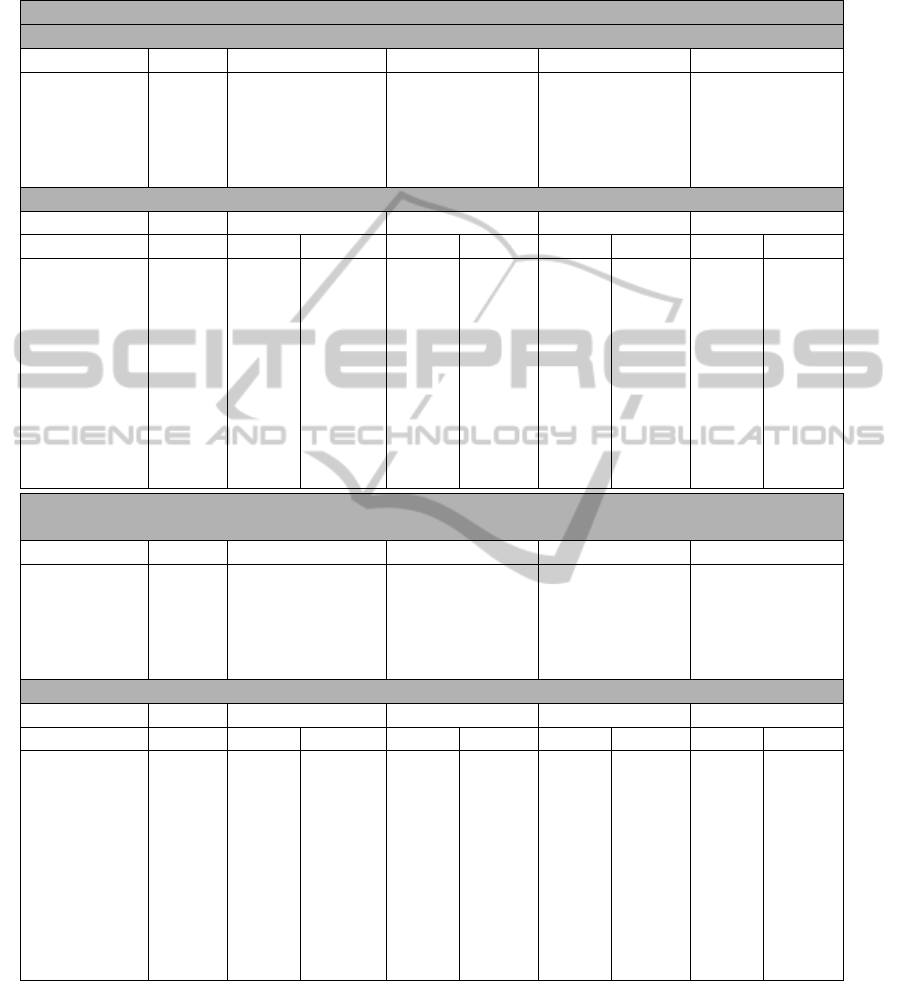
Table 5: MRays/s for Path Tracing and Ambient Occlusion when the sorting is included (inc.) and not included (n.inc.). The
number in parenthesis is the gain in percentage w.r.t. SAH. Bold numbers are the maximum of each row. For secondary and
shadow rays, only columns with the sorting included (inc.) are considered.
Path Tracing
Primary Rays
Scene SAH SPHERE-ORTH SPHERE-OBLI CUBE-ORTH CUBE-OBLI
BUNNY 141.12 147.45(4.29) 144.10(2.06) 144.44(2.29) 143.68(1.77)
F.FOREST 101.70 105.92(3.98) 105.78(3.85) 106.04(4.09) 105.54(3.64)
CONFROOM 149.19 156.16(4.46) 157.52(5.29) 155.91(4.31) 156.78(4.84)
SPONZA 171.75 178.78(3.93) 177.90(3.45) 178.41(3.73) 177.83(3.42)
SIBENIK 143.31 155.06(7.57) 156.16(8.22) 156.66(8.52) 156.83(8.61)
Secondary Rays
Scene SAH SPHERE-ORTH SPHERE-OBLI CUBE-ORTH CUBE-OBLI
n.inc. inc. n.inc. inc. n.inc. inc. n.inc. inc.
BUNNY 36.29 37.14 36.12 38.42 37.33 37.72 36.67 37.33 36.30
(2.27) (-0.47) (5.53) (2.78) (3.77) (1.02) (2.76) (0.01)
F.FOREST 19.36 20.41 20.09 20.62 20.29 20.54 20.22 20.66 20.33
(5.11) (3.61) (6.08) (4.58) (5.73) (4.23) (6.25) (4.75)
CONFROOM 26.21 27.96 27.37 28.11 27.51 28.16 27.57 27.79 27.21
(6.26) (4.25) (6.76) (4.74) (6.94) (4.93) (5.69) (3.67)
SPONZA 26.14 28.47 27.83 28.52 27.91 28.45 27.84 28.73 28.11
(8.16) (6.08) (8.35) (6.34) (8.11) (6.10) (9.01) (7.00)
SIBENIK 19.66 21.72 21.37 21.76 21.40 21.71 21.35 21.76 21.41
(9.46) (7.95) (9.63) (8.12) (9.40) (7.90) (9.64) (8.14)
Ambient Occlusion
Primary Rays
Scene SAH SPHERE-ORTH SPHERE-OBLI CUBE-ORTH CUBE-OBLI
BUNNY 78.72 81.29(3.16) 80.36(2.03) 79.59(1.09) 79.71(1.23)
F.FOREST 63.44 65.09(2.53) 65.09(2.53) 64.92(2.28) 64.85(2.18)
CONFROOM 87.87 94.28(6.79) 94.45(6.96) 93.15(5.66) 94.29(6.80)
SPONZA 112.70 117.33(3.94) 116.82(3.52) 117.11(3.76) 116.32(3.11)
SIBENIK 79.41 83.08(4.40) 84.02(5.48) 83.93(5.38) 84.55(6.07)
Shadow Rays
Scene SAH SPHERE-ORTH SPHERE-OBLI CUBE-ORTH CUBE-OBLI
n.inc. inc. n.inc. inc. n.inc. inc. n.inc. inc.
BUNNY 46.89 48.00 46.33 48.28 46.59 47.04 45.44 47.19 45.58
(2.31) (-1.19) (2.87) (-0.63) (0.32) (-3.18) (0.63) (-2.87)
F.FOREST 30.80 32.02 31.21 32.26 31.45 32.27 31.46 32.23 31.43
(3.79) (1.30) (4.51) (2.07) (4.54) (2.10) (4.43) (1.99)
CONFROOM 52.80 54.88 52.57 54.72 52.43 55.32 52.98 55.11 52.78
(3.77) (-0.44) (3.49) (-0.72) (4.54) (0.32) (4.18) (-0.05)
SPONZA 47.02 50.49 48.65 50.90 49.03 50.65 48.79 50.87 49.00
(6.87) (3.34) (7.62) (4.09) (7.15) (3.62) (7.55) (4.02)
SIBENIK 37.07 39.73 38.58 39.80 38.64 39.96 38.79 39.84 38.68
(6.68) (3.88) (6.83) (4.04) (7.21) (4.42) (6.95) (4.15)
several iterations per camera position.
Kernel Sort is always launched before TI for sec-
ondary rays in PT and shadow rays in AO. In Table 5,
the left columns of each heuristics (tagged with n.inc.)
show the performance of kernel TI, not including the
overload of Sort. On the right columns (tagged with
inc.), the runtime of kernel Sort is taken into account
and added to the runtime of kernel TI. Observe that
this sorting does not affect the results in Table 4.
As it can be seen in Table 4, on average, the
rays that traverse the Multi-kd-trees take less traver-
sal steps to reach their nearest intersection points. We
obtain a gain of up to 14.63% for primary rays and
6.99% for secondary ones in PT, and up to 14.26%
GRAPP 2012 - International Conference on Computer Graphics Theory and Applications
222

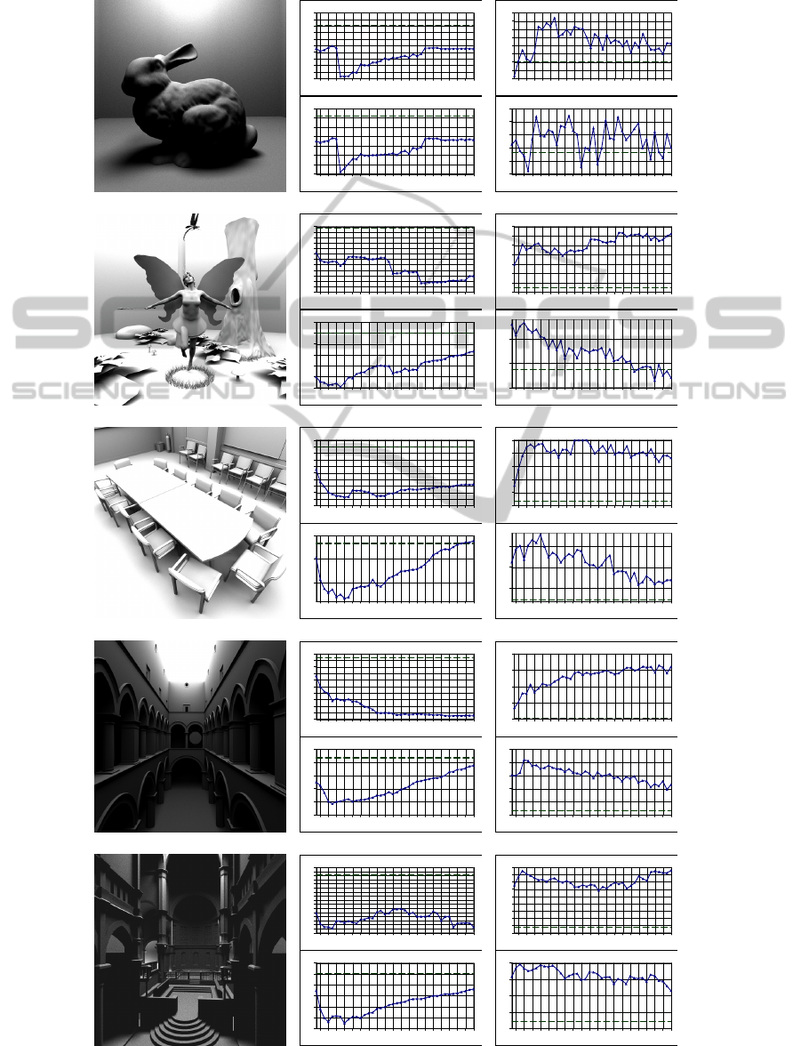
Table 6: Analysis of the COS-ORTH heuristics for Path Tracing w.r.t. traversal steps (middle column) and runtime perfor-
mance (right column).
BUNNY
1,0 3,0 5,0 7,0 9,0 11,0 13,0 15,0 17,0 19,0
Beta
30,0
30,5
31,0
31,5
32,0
32,5
33,0
33,5
34,0
34,5
35,0
Primary Rays
1,0 3,0 5,0 7,0 9,0 11,0 13,0 15,0 17,0 19,0
Beta
29,0
29,5
30,0
30,5
31,0
31,5
32,0
32,5
Secondary Rays
Traversal Steps
1 3 5 7 9 11 13 15 17 19
Beta
141,0
142,0
143,0
144,0
145,0
146,0
147,0
148,0
149,0
Primary Rays
1 3 5 7 9 11 13 15 17 19
Beta
35,5
36,0
36,5
37,0
37,5
38,0
Secondary Rays
MRays/s
FAIRYFOREST
1,0 3,0 5,0 7,0 9,0 11,0 13,0 15,0 17,0 19,0
Beta
43,0
43,5
44,0
44,5
45,0
45,5
46,0
46,5
47,0
47,5
48,0
48,5
49,0
Primary Rays
1,0 3,0 5,0 7,0 9,0 11,0 13,0 15,0 17,0 19,0
Beta
49,0
49,5
50,0
50,5
51,0
51,5
52,0
Secondary Rays
Traversal Steps
1 3 5 7 9 11 13 15 17 19
Beta
101,0
102,0
103,0
104,0
105,0
106,0
107,0
108,0
Primary Rays
1 3 5 7 9 11 13 15 17 19
Beta
19,0
19,5
20,0
Secondary Rays
MRays/s
CONFROOM
1,0 3,0 5,0 7,0 9,0 11,0 13,0 15,0 17,0 19,0
Beta
34,0
34,5
35,0
35,5
36,0
36,5
37,0
37,5
38,0
38,5
39,0
Primary Rays
1,0 3,0 5,0 7,0 9,0 11,0 13,0 15,0 17,0 19,0
Beta
39,0
39,5
40,0
Secondary Rays
Traversal Steps
1 3 5 7 9 11 13 15 17 19
Beta
148,0
150,0
152,0
154,0
156,0
158,0
Primary Rays
1 3 5 7 9 11 13 15 17 19
Beta
26,5
27,0
27,5
Secondary Rays
MRays/s
SPONZA
1,0 3,0 5,0 7,0 9,0 11,0 13,0 15,0 17,0 19,0
Beta
33,0
33,5
34,0
34,5
35,0
35,5
36,0
36,5
37,0
37,5
38,0
Primary Rays
1,0 3,0 5,0 7,0 9,0 11,0 13,0 15,0 17,0 19,0
Beta
39,0
39,5
40,0
40,5
41,0
41,5
Secondary Rays
Traversal Steps
1 3 5 7 9 11 13 15 17 19
Beta
170,0
175,0
180,0
185,0
190,0
Primary Rays
1 3 5 7 9 11 13 15 17 19
Beta
26,0
26,5
27,0
27,5
28,0
28,5
Secondary Rays
MRays/s
SIBENIK
1,0 3,0 5,0 7,0 9,0 11,0 13,0 15,0 17,0 19,0
Beta
38,0
39,0
40,0
41,0
42,0
43,0
44,0
45,0
46,0
Primary Rays
1,0 3,0 5,0 7,0 9,0 11,0 13,0 15,0 17,0 19,0
Beta
45,5
46,0
46,5
47,0
47,5
48,0
48,5
Secondary Rays
Traversal Steps
1 3 5 7 9 11 13 15 17 19
Beta
140,0
142,0
144,0
146,0
148,0
150,0
152,0
154,0
156,0
158,0
Primary Rays
1 3 5 7 9 11 13 15 17 19
Beta
19,5
20,0
20,5
21,0
21,5
Secondary Rays
MRays/s
IMPROVING RAY TRAVERSAL BY USING SEVERAL SPECIALIZED KD-TREES
223

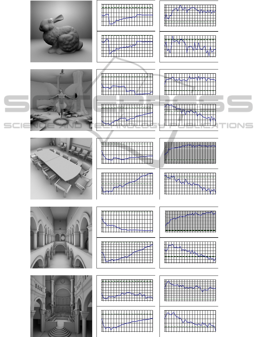
Table 7: Analysis of the COS-ORTH heuristics for Ambient Occlusion w.r.t. traversal steps (middle column) and runtime
performance (right column).
BUNNY
1,0 3,0 5,0 7,0 9,0 11,0 13,0 15,0 17,0 19,0
Beta
30,0
31,0
32,0
33,0
34,0
35,0
Primary Rays
1,0 3,0 5,0 7,0 9,0 11,0 13,0 15,0 17,0 19,0
Beta
25,5
26,0
26,5
27,0
27,5
28,0
28,5
29,0
Secondary Rays
Traversed Rays
1,0 3,0 5,0 7,0 9,0 11,0 13,0 15,0 17,0 19,0
Beta
78,0
78,5
79,0
79,5
80,0
80,5
81,0
81,5
82,0
Primary Rays
1,0 3,0 5,0 7,0 9,0 11,0 13,0 15,0 17,0 19,0
Beta
44,5
45,0
45,5
46,0
46,5
47,0
47,5
Secondary Rays
MRays/s
FAIRYFOREST
1,0 3,0 5,0 7,0 9,0 11,0 13,0 15,0 17,0 19,0
Beta
44,0
45,0
46,0
47,0
48,0
49,0
50,0
Primary Rays
1,0 3,0 5,0 7,0 9,0 11,0 13,0 15,0 17,0 19,0
Beta
40,5
41,0
41,5
42,0
42,5
43,0
Secondary Rays
Traversed Rays
1,0 3,0 5,0 7,0 9,0 11,0 13,0 15,0 17,0 19,0
Beta
63,0
63,5
64,0
64,5
65,0
65,5
Primary Rays
1,0 3,0 5,0 7,0 9,0 11,0 13,0 15,0 17,0 19,0
Beta
29,5
30,0
30,5
31,0
31,5
Secondary Rays
MRays/s
CONFROOM
1,0 3,0 5,0 7,0 9,0 11,0 13,0 15,0 17,0 19,0
Beta
34,0
35,0
36,0
37,0
38,0
39,0
Primary Rays
1,0 3,0 5,0 7,0 9,0 11,0 13,0 15,0 17,0 19,0
Beta
30,6
30,8
31,0
31,2
31,4
31,6
31,8
32,0
Secondary Rays
Traversed Rays
1,0 3,0 5,0 7,0 9,0 11,0 13,0 15,0 17,0 19,0
Beta
86,0
87,0
88,0
89,0
90,0
91,0
92,0
93,0
94,0
95,0
96,0
97,0
98,0
Primary Rays
1,0 3,0 5,0 7,0 9,0 11,0 13,0 15,0 17,0 19,0
Beta
50,0
50,5
51,0
51,5
52,0
52,5
53,0
53,5
Secondary Rays
MRays/s
SPONZA
1,0 3,0 5,0 7,0 9,0 11,0 13,0 15,0 17,0 19,0
Beta
33,0
34,0
35,0
36,0
37,0
38,0
Primary Rays
1,0 3,0 5,0 7,0 9,0 11,0 13,0 15,0 17,0 19,0
Beta
32,8
33,0
33,2
33,4
33,6
33,8
34,0
34,2
34,4
Secondary Rays
Traversed Rays
1,0 3,0 5,0 7,0 9,0 11,0 13,0 15,0 17,0 19,0
Beta
112,0
113,0
114,0
115,0
116,0
117,0
118,0
119,0
120,0
121,0
122,0
Primary Rays
1,0 3,0 5,0 7,0 9,0 11,0 13,0 15,0 17,0 19,0
Beta
46,0
46,5
47,0
47,5
48,0
48,5
49,0
49,5
Secondary Rays
MRays/s
SIBENIK
1,0 3,0 5,0 7,0 9,0 11,0 13,0 15,0 17,0 19,0
Beta
40,0
41,0
42,0
43,0
44,0
45,0
46,0
47,0
48,0
Primary Rays
1,0 3,0 5,0 7,0 9,0 11,0 13,0 15,0 17,0 19,0
Beta
37,5
38,0
38,5
39,0
39,5
40,0
Secondary Rays
Traversed Rays
1,0 3,0 5,0 7,0 9,0 11,0 13,0 15,0 17,0 19,0
Beta
79,0
79,5
80,0
80,5
81,0
81,5
82,0
82,5
83,0
83,5
84,0
84,5
85,0
Primary Rays
1,0 3,0 5,0 7,0 9,0 11,0 13,0 15,0 17,0 19,0
Beta
36,5
37,0
37,5
38,0
38,5
39,0
Secondary Rays
MRays/s
GRAPP 2012 - International Conference on Computer Graphics Theory and Applications
224

for primary and 8.55% for shadow rays in AO. Pri-
mary rays in PT and AO are almost identical, so their
results are very similar. Shadow rays in AO take fewer
traversal steps than secondary rays in PT. This makes
sense because the average length of shadow rays in
AO is shorter than that of secondary rays in PT.
Concerning the execution model of GPUs, the
traversal of different rays is not totally independent
from each other. Therefore, texture cache misses and
divergences can make the runtime execution differ-
ent than expected. Even primary rays suffer from
these stalls since the decrease in traversal steps do
not agree with the improve in performance. For in-
stance, SPHERE-ORTH takes 11.08% less traversal
steps than SAH for BUNNY in PT (Table 4), but it
only reaches an improvement of 4.29% in perfor-
mance (Table 5). On the contrary, this clear differ-
ence does not hold for secondary rays. It is true that
the sorting can entail an increase of their coherence,
but secondary rays are randomly spawned and sort-
ing only considers the kd-tree selection. Thus, reports
highly depend on how these rays are concretely built
during rendering.
Regarding sorting, the performance of our heuris-
tics exceeds that of SAH when the overload due to
sorting is not considered (columns n.inc. in Table
5). When this overload is included (columns inc.)
our heuristics keep overcoming in most cases. The
overload is more relevant in AO since shadow rays
traverse fewer steps on average. Notice that scenes
BUNNY and CONFROOM have the lowest average
traversal steps and their results show that the overload
make their runtime performance mostly slower w.r.t.
SAH.
We have also compared SAH with the cosine
heuristics. The settings are the same than previous
heuristics. We have measured the traversal steps and
the runtime performance (including Sort) by ranging
β from 0.5 to 20 in steps of 0.5. Tables 6 and 7 show
the results for COS-ORTH (blue curves) for PT and
AO, respectively. The results for COS-OBLI are not
depicted because they have a similar behaviour. A
dashed horizontal line is added to the charts to com-
pare this heuristics with SAH.
With respect to traversal steps in PT, it can be seen
a decrease of them as β increases until it reaches a
value between 2 and 3.5, for primary and secondary
rays. These values of β lead to similar weights re-
garding the spherical and cubic heuristics. After that,
the behaviour of rays becomes scene-dependant. The
charts of runtime performance have an inverse be-
haviour, since the fewer traversal steps the rays tra-
verse, the higher the runtime performance is.
The charts of traversal steps for primary and
shadow rays have a similar shape in AO. Again, the
steps traversed by shadow rays are fewer than those
for secondary rays in PT due to their shorter length.
Comparing the performance charts between PT
and AO, AO exhibits a better performance than PT,
but the difference between COS-ORTH and SAH is
larger for PT (Table 6) than for AO (Table 7). The
explanation of this is the same as previous heuristics,
i.e. the constant overload of sorting is more relevant
for those rays with fewer traversal steps.
8 CONCLUSIONS AND
FUTURE WORK
In this paper, we have presented six new heuristics de-
veloped from a mathematical description of the orig-
inal SAH. These heuristics specialize SAH for differ-
ent sets of ray directions by restricting their domain or
assuming different probabilities. In order to cover the
whole space of directions, several sets have been pro-
posed and a kd-tree has been built for each of them
(Multi-kd-tree). The traversal of a Multi-kd-tree re-
ports fewer traversal steps and better runtime perfor-
mance than a single SAH-based kd-tree over usual
scenes.
However, runtime performance does not agree
with the number of traversal steps, due to the execu-
tion on SIMT hardware. This fact is even more rele-
vant for secondary or shadow rays due to their random
spawning. It is necessary further research about this
issue to fill the gap between traversal steps and run-
time performance on parallel hardware.
A tighter division of the direction space could be
realized. However, two considerations must be taken
into account. First, all the information needed for the
traversal has to be stored in device memory. So, a big-
ger amount of divisions entails more memory require-
ments. Second, the selection of the kd-tree to traverse
has to be quick. In this work, only few comparisons
are needed, which makes the selection negligible with
respect to the whole traversal.
Finally, the cosine heuristics have been devel-
oped independently to the spherical and cubic heuris-
tics. It would be interesting to analyze the behaviour
of spherical or cubic patches in which rays are dis-
tributed according to the cosine heuristics.
ACKNOWLEDGEMENTS
This paper has been supported by the Spanish projects
CCG10-UCM/TIC-5476 and GR35/10-A-921547.
IMPROVING RAY TRAVERSAL BY USING SEVERAL SPECIALIZED KD-TREES
225

Thanks to The Stanford 3D Scanning Repository
for the BUNNY model, The Utah 3D Animation
Repository for the FAIRYFOREST scene and Marko
Dabrovic for the SIBENIK and SPONZA scenes.
REFERENCES
Aila, T. and Laine, S. (2009). Understanding the Efficiency
of Ray Traversal on GPUs. In High-Performance
Graphics 2009, pages 145–149.
Bittner, J. and Havran, V. (2009). RDH: Ray Distribution
Heuristics for Construction of Spatial Data Structures.
In SCCG 2009, pages 61–67, Budmerice, Slovakia.
Fabianowski, B., Flower, C., and Dingliana, J. (2009). A
Cost Metric for Scene-Interior Ray Origins. In Euro-
graphics 2009 Short Papers, pages 49–52.
Foley, T. and Sugerman, J. (2005). KD-Tree Acceleration
Structures for a GPU Raytracer. In Graphics Hard-
ware 2005, pages 15–22.
Garanzha, K. and Loop, C. (2010). Fast Ray Sorting and
Breadth-First Packet Traversal for GPU Ray Tracing.
In Eurographics 2010.
Goldsmith, J. and Salmon, J. (1987). Automatic Creation of
Object Hierarchies for Ray Tracing. IEEE Computer
Graphics and Application, 7(5):14–20.
G
¨
unther, J., Popov, S., Seidel, H.-P., and Slusallek, P.
(2007). Realtime Ray Tracing on GPU with BVH-
based Packet Traversal. In Eurographics Symposium
on Interactive Ray Tracing 2007, pages 113–118.
Harris, M., Owens, J. D., Sengupta, S., Tseng, S., Zhang,
Y., Davidson, A., and Satish, N. (2010). CUDA
Data Parallel Primitives Library (CUDPP 1.1.1).
http://code.google.com/p/cudpp/.
Havran, V. (2000). Heuristic Ray Shooting Algorithms.
Ph.d. thesis, Faculty of Electrical Engineering, Czech
Technical University in Prague.
Havran, V. and Bittner, J. (1999). Rectilinear Trees for Pre-
ferred Ray Sets. In SCCG 1999, pages 171–178, Bud-
merice, Slovakia.
Horn, D. R., Sugerman, J., Mike, H., and Hanrahan, P.
(2007). Interactive KD-Tree GPU Raytracing. In I3D
2007, pages 167–174.
Hunt, W. and Mark, W. R. (2008). Adaptive Acceleration
Structures in Perspective Space. In IEEE Symposium
on Interactive Ray Tracing, pages 11–17.
MacDonald, D. J. and Booth, K. S. (1990). Heuristics for
ray tracing using space subdivision. Visual Computer,
6(3):153–166.
Pharr, M. and Humphreys, G. (2010). Physically Based
Rendering: From Theory to Implementation (second
edition). Morgan Kaufmann.
Popov, S., G
¨
unther, J., Seidel, H.-P., and Slusallek, P.
(2007). Stackless KD-Tree Traversal for High Perfor-
mance GPU Ray Tracing. Computer Graphics Forum
(Proceedings of Eurographics), 26(3):415–424.
Thrane, N., Simonsen, L. O., and Orbaek, A. P. (2005). A
Comparison of Acceleration Structures for GPU As-
sisted Ray Tracing. Technical report, University of
Aarhus.
Torres, R., Martin, P. J., and Gavilanes, A. (2011). Travers-
ing a BVH Cut to Exploit Ray Coherence. In GRAPP
2011, pages 140–150.
Torres, R., Mart
´
ın, P. J., and Gavilanes, A. (2009). Ray cast-
ing using a roped BVH with CUDA. In Proc. Spring
Conference on Computer Graphics, pages 107 – 114.
Wald, I. (2007). On Fast Construction of SAH-Based
Bounding Volume Hierarchies. In Symposium on In-
teractive Ray Tracing 2007, pages 33–40.
Wald, I. and Havran, V. (2006). On Building Fast KD-Trees
for Ray Tracing, and on Doing That in O(NlogN). In
Symposium on Interactive Ray Tracing, pages 61–69.
GRAPP 2012 - International Conference on Computer Graphics Theory and Applications
226