
GROUP-WISE SPARSE CORRESPONDENCES BETWEEN
IMAGES BASED ON A COMMON LABELLING APPROACH
Albert Solé-Ribalta
1
, Gerard Sanromà
1
, Francesc Serratosa and René Alquézar
2
1
Departament d’Enginyeria Informàtica i Matemàtiques, Universitat Rovira i Virgili, Tarragona, Spain
2
Institut de Robtica i Informàtica Industrial, CSIC-UPC, Barcelona, Spain
Keywords: Multiple Point Set Alignment, Group Wise Point Set Alignment.
Abstract: Finding sparse correspondences between two images is a usual process needed for several higher-level
computer vision tasks. For instance, in robot positioning, it is frequent to make use of images that the robot
captures from their cameras to guide the localisation or reduce the intrinsic ambiguity of a specific
localisation obtained by other methods. Nevertheless, obtaining good correspondence between two images
with a high degree of dissimilarity is a complex task that may lead to important positioning errors. With the
aim of increasing the accuracy with respect to the pair-wise image matching approaches, we present a new
method to compute group-wise correspondences among a set of images. Thus, pair-wise errors are
compensated and better correspondences between images are obtained. These correspondences can be used
as a less-noisy input for the localisation process. Group-wise correspondences are computed by finding the
common labelling of a set of salient points obtained from the images. Results show a clear increase in
effectiveness with respect to methods that use only two images.
1 INTRODUCTION
Determining sparse correspondences between sets of
features is a recurrent problem in computer vision. It
arises at the early stages of many computer vision
applications such as 3D scene reconstruction, object
recognition, pose recovery and image retrieval,
among others. Therefore, it is of basic importance to
develop methods that are both effective -in the sense
of not being prone to local optima- and robust -in the
sense of being able to accommodate a wide range of
image deformations as well as noisy measurements-.
We divide classical approaches to compute pair-wise
correspondences into: (1) correlation-based
strategies that compute the matches by means of the
similarity between the image patches around some
interest points (Harris and Stephens 1988) and; (2)
approaches based on feature-descriptors that use
local information at the interest points to compute
descriptor-vectors (Mikolajczyk and Schmid 2005).
The use of local image contents may not suffice to
get a reliable correspondence between points of two
images under certain circumstances e.g. large
rigid/non-rigid deformations. This is the case of the
model fitting paradigm RANSAC (Fischler and
Bolles 1981) which is extensively used in computer
vision to reject outliers or the Iterative Closest Point
(ICP) method (ZHANG 1992) that attempt to
simultaneously solve the correspondence and the
alignment problem. All the mentioned approaches
suffer from two major drawbacks. On the one hand,
most of these optimization strategies rely on
reasonable initial guesses in order to find the global
optimum. On the other hand, if there is too much
deformation between both images, their underlying
geometrical models may fail to accommodate the
transformation relating them, even under a
reasonable initial guess.
To solve the aforementioned drawbacks, we face
the correspondence problem in a group-wise
manner. In this way, the flow of information among
the pair-wise relations of the group has several
advantages. It helps to constrain the search of our
method towards a globally convenient direction.
This contributes to avoid poor local optima. And, in
addition it alleviates the limitations inherent to the
geometrical models. To complement the method, we
develop effective mechanisms to detect outlying
points between two point-sets whose effects are
conveniently propagated to the rest of the group.
The approach we propose has been successfully
applied to graph matching (Solé-Ribalta
269
Solé-Ribalta A., Sanromà G., Serratosa F. and Alquézar R..
GROUP-WISE SPARSE CORRESPONDENCES BETWEEN IMAGES BASED ON A COMMON LABELLING APPROACH.
DOI: 10.5220/0003846802690278
In Proceedings of the International Conference on Computer Vision Theory and Applications (VISAPP-2012), pages 269-278
ISBN: 978-989-8565-03-7
Copyright
c
2012 SCITEPRESS (Science and Technology Publications, Lda.)
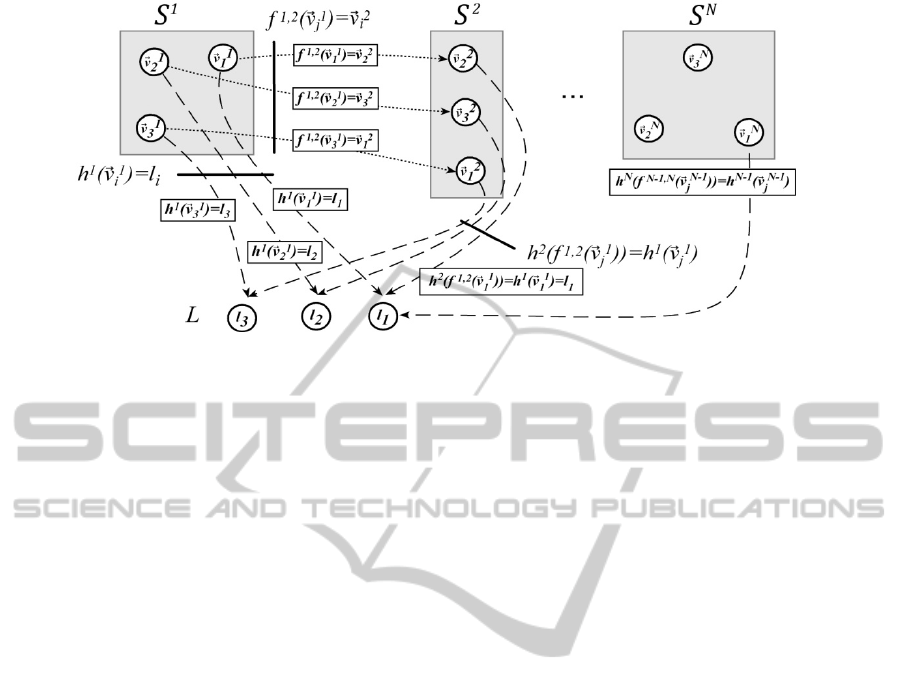
Figure 1: Example of common labelling.
and Serratosa 2010). Here, we adapt the graph-
oriented solution to group-wise point registration
and we enhance its effectiveness incorporating a
geometrical model and an outlier detection
mechanism.
Several similar solutions have been proposed for
graph matching purposes. We highlight (Williams,
Wilson et al. 1997) where some pair-wise matchings
where induced using Bayesian inference. The main
limitation of the methodology is that is not
applicable to more than 3 graphs. Another solution,
also applied to graphs, was proposed in (Solé-
Ribalta and Serratosa 2011). In this case the
extension to multiple graphs is straightforward;
however, its high computational cost makes it again
not applicable with more than 3 graphs.
Related to the field of group-wise point
registration when data is a sparse set of points we
next highlight the following work. In (Fergus,
Perona et al. 2007) a method to learn objects and
detect parts of objects is presented. The model is
learned taking images that represent the selected
object from the same point of view and without
background. The method does not explicitly address
the problem presented here due to the aim is to
construct a model for object recognition. Another
related work is presented in (Wang, Vemuri et al.
2008), which performs alignment of sparse data
points taking into account that points contain non-
rigid deformation. The most similar method to the
one we present could be (Cootes, Twining et al.
2010). It is based on group-wise point set
correspondence but it has no consideration about
outlier detection, which makes its applicability not
feasible with the concrete problem we present. This
last work was evaluated using two hand-made
labelled data sets.
The article is structured as follows. Section 2
gives some basic definitions. Section 3 and 4
describes the method used to deduct the group-wise
correspondences. Section 3 describes the common
labelling framework and section 4 describes the cost
function as well as the outlier detection procedure.
Section 5 describes the optimization algorithm.
Section 6 evaluates the new method and Section 7
concludes the paper.
2 BASIC DEFINITIONS
Let
={
,
,..
}
be a set of points with
elements. In our method, these types of sets
represent images and their elements are salient
points extracted from them. Moreover, we represent
the set of images by the set Γ={S
1
, S
2
, …, S
N
}. Each
in Γ is the characterisation of an image.
Following this notation, the correspondence between
salient points of a set of images are characterised by
the labellings between the elements of the sets
in
Γ. Note that outlier points in images are also
represented as elements in S
p
. These outlier points in
the images do not correspond to other points on the
other images and so the corresponding elements in
the sets have not to be labelled from or to these
elements.
Definition 1. Labelling between two sets of points:
Given two sets of points
={
,
,..,
}
and
={
,
,..,
} with
and
elements, a
labelling between these sets assign elements of the
first set to elements of the second set
=
. We
represent this labelling in a binary matrix as follows,
VISAPP 2012 - International Conference on Computer Vision Theory and Applications
270

=
1
=
0ℎ
(1)
Definition 2. Multiple Labelling between sets of
points. Let Γ={S
1
, S
2
, …, S
N
} be a set of N sets of
points, each with a concrete number of elements
,
:1... The set φ is a Multiple Labelling of Γ if it
contains one and only one labelling between any
pair of set of points, =
{
,
,…,
,
,…,
,
}
.
Some inconsistencies may appear in the multiple
labelling if these labellings are obtained by only
considering the set of points they relate. Fig. 2.a and
Fig. 2.b shows an example of an inconsistent and
Figure 2.a: Example of inconsistent multiple labelling.
Figure 2.b: Example of consistent multiple labelling.
consistent multiple labelling respectively. In the
inconsistent labelling point
is labelled to
by
function
,
and it is labelled to
by
,
.
However,
,
labels
to
. Therefore, there is
no a global correspondence between the salient
points in the original images. See how this is fixed in
the consistent multiple labelling.
Some methods solve this problem by first
finding the pair-wise labelling to next redefining
them with the aim of eliminating inconsistencies
(Bonev, Escolano et al. 2007). The main property of
our method is that it obtains directly a multiple
labelling. That is, it considers from the first moment
the group-wise correspondences, and so,
inconsistencies cannot appear due to our
methodology.
We say that a multiple labelling is consistent if
there are not any inconsistencies. That is, it fulfils
that,
,
,
=
,
,
0<,,≤,0<≤
(2)
When the sets of points in Γ form a Consistent
Multiple Labelling, it is possible to define a
Common Labelling. It represents a Multiple
Labelling in a compact way and forms the basis of
the proposed algorithm.
Definition 3. Common Labelling (CL) of sets of
points. Let be a Consistent Multiple Labelling of
Γ. Let be a virtual point set. The Common
Labelling =
{
ℎ
,ℎ
,…,ℎ
}
is defined to be a set
of bijective mappings from the points of Γ to as
follows:
ℎ
(
)
=,ℎ
=ℎ
,
1
≤
,
≤
,2
≤
≤
,
,
(
)=
(3)
Figure 1 shows the relation between a Consistent
Multiple Labelling and a Common Labelling.
3 COMMON LABELLING
FRAMEWORK
Given two sets of salient points,
and
,
extracted from two images, to bring the problem to
the continuous domain we relax the matches
between these point sets i.e. (1). To this aim, we
represent the probability of labelling
to
in
matrix from as:
,
[
,
]
=(
,
=
)
(4)
Moreover, we consider the probability of
labelling point
of set
to a virtual point
is the
probabilistic union of all the paths that go through
the points of a third set
. That is,
[
,
]
=ℎ
=
=
=
,
=
⋂ℎ
=
(5)
Combining (5) with P
f
definitions and assuming
independence of events we get:
[
,
]
=
,
[
,
]
·
[
,
]
=
,
·
(6)
In a similar way, we could infer that:
,
=
·
(7)
Due to our final objective is to compute a CL, our
new energy function depends on the probabilities
GROUP-WISE SPARSE CORRESPONDENCES BETWEEN IMAGES BASED ON A COMMON LABELLING
APPROACH
271

instead of
. To this aim, we define the energy of a
group-wise point alignment as:
=
−
[
,
]
·
[
,
]
≡
,
[,]
·
[
,
]
·
[
,
]
≡
,
[,]
·
,
,
(8)
Energy of (8) is a generalization of energy of pair-
wise labellings.
Reorganizing (8) we can easily see the influence
of matchings
→
over
→
:
=
−
[
,
]
·
[
,
]
≡
,
[,]
[
,
]
·
[
,
]
≡
,
[,]
·
,
,
(9)
This influence is identified as
in (9) and will be
described in detail in section 4.
4 PAIR-WISE COMPATIBILITY
COEFFICIENTS
Given two sets of points
={
,
,..,
} and
={
,
,..,
}, where
=
,
and
=
,
, contain the column vectors of the
two-dimensional coordinates (horizontal and
vertical) of each point, in this section we will
describe the details of the computation of the
compatibility coefficients
,
appearing under
equation (9).
This quantity
, also known as the support
function, is addressed at measuring the support for
the match
→
received from the rest of the
matches
→
. This is a common strategy
followed in the probabilistic relaxation approaches
(Rosenfeld, Hummel et al. 1976; Hummel and
Zucker 1983).
The main idea underpinning our computation of
the support function is that two points
and
from two graphs and are in correspondence as
long as they show similar spatial distributions in
comparison to the rest of the points around them.
Geometric evidence is widely used to solve the
correspondence problem. In order to be robust to
arbitrary initial poses of the point-sets under a
certain geometric assumption we need to include the
estimation of the alignment parameters into the
problem. Thus we redefine the support function in
the following way
=max
,
[
,
]
·
,
(Φ
)
(10)
where
,
[
,
]
corresponds to the globally
propagated probability to match nodes , of graphs
, and
,
(Φ
) is the compatibility of the
simultaneous matches
→
and
→
given
the affine parameters Φ
.
In this new formulation, we attain robustness to
affine pose of the point-sets by selecting the pose
configuration that leads to the maximum support.
With respect to classical point-set registration
methods, our approach has the particularities that it
is aimed at multiple point-set registration and that
alignment parameters are local to each
correspondence hypothesis
⟶
instead of
being a property global to all the points in the set.
Since we compare relational geometric
measurements, we define the new coordinate vectors
=
−
and
=
−
, that
represent the coordinates of the points
and
relative to
and
, respectively.
We define the compatibility between two
relational geometric measurements
and
under the action of the affine parameters Φ
as:
,
(
Φ
)
=−
−Φ
(11)
where Φ
is a 22 non-singular matrix of affine
transformation parameters (note that
and
are
already invariant to translation),
‖
·
‖
is the squared
Mahalanobis distance with covariance matrix Σ, and
is a thresholding quantity that controls the outlier
process whose estimation will be detailed in the next
section.
According to the proposed measure, the more
dissimilar are the relations, the lower is their
compatibility. The scale of this comparison is
VISAPP 2012 - International Conference on Computer Vision Theory and Applications
272

effectively controlled by the matrix
Σ=
0
0
, a
diagonal matrix of variances which may be
empirically estimated from the data.
With these ingredients, the optimal
transformation parameters Φ
∗
that maximize
equation (10) are:
Φ
∗
=min
,
[
,
]
−Φ
Σ
−Φ
(12)
where
Φ
∗
=
. We have discarded the
constant quantities not depending on the alignment
parameters. Note that we have turned the
maximization into a minimization by reversing the
sign.
Consider the following residuals from the
alignment of points
and
.
=
−
+
=
−
+
(13)
Then, the objective function of equation (12) is
equivalent to the following expression:
ℱ=
,
[,
]
+
(14)
Taking derivatives of ℱ with respect to Φ
we
obtain the following expressions:
ℱ
=−
,
[,
]
2
ℱ
=−
,
[
,
]
2
ℱ
=−
,
[
,
]
2
ℱ
=−
,
[,]
2
(15)
The optimal transformation parameters Φ
∗
are
found by solving the set of equations:
ℱ
=0,…,
ℱ
=0,
(16)
with respect to the parameters. This linear system
can be expressed in matrix form =
, where
is a 44 matrix and
=
11
,
12
,
21
,
22
and
are 4-column-vectors. This can be solved by matrix
inversion (i.e.,
=
−1
).
4.1 Outlier Detection
According to our purposes, a point
∈
(or
∈
) is considered an outlier as far as there is no
point
,∀∈1..
|
|
(or
,∀∈1..
|
|
) which
presents a support
(10) above a given threshold.
Substituting the compatibilities of equation (11)
into equation (10), the final expression for the
supports is:
=
,
[,]−
−Φ
∗
(17)
where Φ
∗
are the optimal transformation parameters
computed using equation (12).
The parameter plays the role of the robustness
parameter used by (Rangarajan, Chui et al. 1997;
Gold, Rangarajan et al. 1998). It controls whether
the geometrical compatibility term contributes either
positively (i.e., <
−Φ
∗
) or negatively
to the support measure.
We model the outlier detection process as an
assignment to (or from) a special point. This is
similar to null vertex assignments in (Wong and You
1985). We consider as outliers all the assignments
⟶
such that
,
<0.
The threshold represents the quantity from
which the compatibility starts to contribute
negatively. Therefore, it seems reasonable to express
in terms of a squared Mahalanobis distance, i.e.
=
. If we express the threshold distance
vector proportionally to the standard deviations of
the data, i.e.
=
(
,
)
, the expression of
becomes
=
Σ
=
+
=2
(18)
considering that Σ matrix is diagonal.
Rangarajan et al. (Rangarajan, Chui et al.
1997; Gold, Rangarajan et al. 1998) do not address
the estimation of this parameter in their paper. On
the contrary, we define as a function of the
number of standard deviations permitted in the
registration errors, in order to consider a relation
plausible.
GROUP-WISE SPARSE CORRESPONDENCES BETWEEN IMAGES BASED ON A COMMON LABELLING
APPROACH
273

5 THE ALGORITHM
Considering the optimization function in (9) for
multiple point set matching, we focus on substituting
to it the support function deduced in section 4.
The problem becomes then one of joint
estimation of correspondence and alignment
parameters in which the recovery of the
correspondences is influenced by the pose of the
point-sets and vice-versa. Most point-set registration
methods consist of an iterative process that
alternates alignment and correspondence updates.
Several approaches exist in order to solve this
chicken-and-egg problem as, for example, the well-
known ICP (ZHANG 1992), Robust Point Matching
(RPM) (Rangarajan, Chui et al. 1997; Gold,
Rangarajan et al. 1998) or the Expectation-
Maximization Algorithm (Jian and Vemuri 2005;
Myronenko and Song 2010; Horaud, Forbes et al.
2011; Jian and Vemuri 2011).
To optimize our objective function we propose to
use a similar dual step solution based on first
maximize the point alignment to later maximize the
correspondences. We base our method on the
Graduated assignment (Gold and Rangarajan 1996).
In this way, we approximate
with Taylor series
expansion considering that the point alignment given
by Φ
∗
is already optimized. Similarly to (Gold and
Rangarajan 1996) we deduce that minimizing
function (9) is equivalent to maximizing:
{
}
=
,
·
[
,
]
(19)
where,
,
=
[
,
]
[
,
]
·
[
,
]
·
,
,
(20)
Equation (20) reduces the problem to the
quadratic assignment problem, where is the cost
matrix and represents a stochastic matrix
(Sinkhorn 1964) that encode the assignment
probabilities.
The original procedure to optimize equation (20)
is the following: start with a valid
, compute
cost matrix
, apply Graduated Assignment to
compute next
and start again until
convergence is reached.
Similarly, in our objective function to maximize
the common labelling assignments we focussed in
P
as (8) and (9) indicates. In addition, we are
required to maximize the alignment to compute the
compatibility cost. So, our proposed maximization
procedure has the following steps: start with a valid
, maximize alignment with respect to the rest of
points (12), compute cost matrix
using costs in
(10), apply Graduated Assignment to compute next
and start again until convergence is reached.
An outline of the procedure is given below.
Program MSP-Aligment inputsΓ returns
=
=2
Loop A: (Do A until ≥
)
=0
Loop B: (Do B until Q converges or <
)
,
=
(
,,,
,Γ
)
=
·
=ℎ(
)
=+1
End B
=∗
End A
End Program
where
,
,
and
correspond to the parameters
of (Gold and Rangarajan 1996) and are application
dependant. In our case, we used the values proposed
in the original article. Function
computes optimizes the alignments and the point-to-
point assignations, an outline of the procedure is
given below:
Function input
,,,
,Γ
returns
,
For ∀∈1..
|
Γ
|
,≠
,
=
·
For =1..
|
|
For =1..
|
|
,≠
For =1..
|
|
,≠
,
=
,
+
[
,
]
·
·
,
[
.
]
·−
−Φ
∗
End
End
End
End
End Function
Taking into account our definition of outlier
detection, we require to adapt the Sinkhorn
normalization (Sinkhorn 1964) to consider them.
VISAPP 2012 - International Conference on Computer Vision Theory and Applications
274
Recall first that the resulting
,
could be negative
values, however after the exponentiation all values
become strictly positive and therefore we can
assume the Sinkhorn normalization can be applied.
In the normalization over matrix
, we keep in
mind that outliers are special assignation that only
satisfy one-way constraints, in this way we can
easily consider several points as outliers. To this
aim, we enhance each matrix
with an extra row
and column, following a similar procedure than the
slacks in (Gold and Rangarajan 1996). We initialize
these extra row and column with the value of 1. We
aim to detect outliers, that is points which have
<0∀ or . We know that
≥1 if ≥0,
thus we expect points which have all possible
assignations negative are assigned to this special row
or column. Finally, when the Sinhorn method has
finished the extra row and column are removed
leading to the resulting matrices of global
assignments
.
Note that now
cannot be theoretically
considered a probability assignation matrix, due to
∑
[,]≠1
, neither for rows nor for columns.
However, we still can ensure that
∑
[,]<1
and that each individual value is positive. So, what
was a probability matrix
, now it can be assumed
to be a fuzzy assignation matrix.
6 EVALUATION
We evaluate the effectiveness of the presented
method in a series of group-wise image registration
experiments. We use real images from the database
in (Mikolajczyk, Tuytelaars et al. 2011). Feature
points from each image have been extracted using
the Harris operator (Harris and Stephens 1988). We
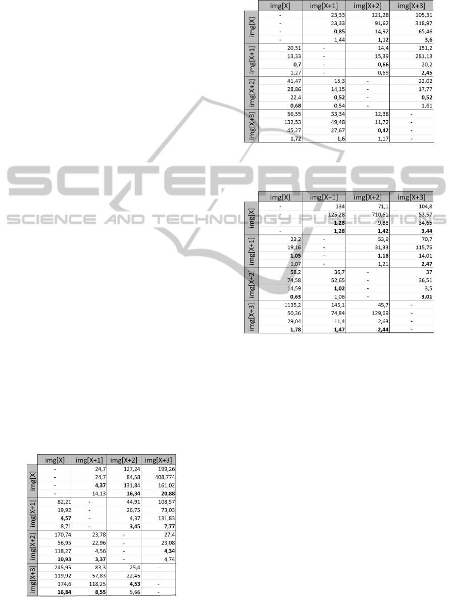
Table 1: Results using New York. We have used 25
groups of N=4 images (i.e., results are averaged over 25
experiments).
Table 2: Results using Van Gogh. We have used 14
groups of N=4 images (i.e., results are averaged over 14
experiments).
Table 3: Results using Asterix. We have used 17 groups of
N=4 images (i.e., results are averaged over 17
experiments).
use the following datasets: New York, Van Gogh
and Asterix. Each dataset is composed by an ordered
sequence of images from the same scene showing
increasing levels of zoom or zoom plus rotation.
Each test is performed on a group of N images. We
compare the following four methods. (1) Pairwise
ICP+RANSAC, which applies the well-known
ensemble ICP+RANSAC between each pair of
images. (2) Confident ICP+RANSAC, which
computes the labellings between only the most
similar pairs and infers the rest by composition (this
method exploits the prior knowledge about the
underlying order of the images). A very similar
strategy is used in (Williams, Wilson et al. 1997).
(3) Pairwise Labelling, which applies the proposed
approach independently to each pair of images and
(4) Group-wise Labelling, which applies the
proposed approach jointly to all the images of the
group. This method is the prime motivation of our
work. When comparing the last two methods, it is
our aim to elucidate the benefits of the group-wise
approach vs. the pairwise one. All the methods have
GROUP-WISE SPARSE CORRESPONDENCES BETWEEN IMAGES BASED ON A COMMON LABELLING
APPROACH
275

been initialized with the results of the matching by
correlation. Regardless the labellings are computed
in either pair-wise or a group-wise fashion, results
are evaluated in a pair-wise basis. We use the DLT
algorithm (Kovesi 2009) to compute the
homography corresponding to a given labelling
between two images. Since ground truth
homographies are available, we measure the
accuracy through the mean projection error (MPE)
in pixels.
Tables 1, 2 and 3 show the results of the New
York, Van Gogh and Asterix datasets using groups
of N=4 images. From top to bottom, each cell
contains the MPE of Pair-wise ICP+RANSAC,
Confident ICP+RANSAC, Pair-wise Labelling and
Group-wise Labelling. Images are arranged in the
rows and columns of the tables according to their
logical order. The diagonal cells are empty since
they correspond to self-labellings.
Analyzing the results, we see that the common
labelling approach obtains usually the lowest mean
projection error.
This fact is clear with distant images; see for
instance row[] and [+3] where in all
datasets the common labelling error is much lower
with respect to all other methods. In some cases,
with adjacent images the pair-wise labelling method
obtains better labellings, e.g. row [+3] and
column [+2] of Table 1. However, the
difference between this method and the common
labelling method is low, recall that the mean
projection error is in pixels.
In addition to MPE, we show three concrete
examples (Figs. 3, 4, 5, 6, 7 and 8) of labellings
obtained with the pair-wise method and the common
Figure 3: Concrete labelling example of Asterix dataset
using obtained using pair-wise method.
Figure 4: Concrete labelling example of Asterix dataset
using obtained using common labelling method.
Figure 5: Concrete labelling example of New York dataset
using obtained using pair-wise method.
Figure 6: Concrete labelling example of New York dataset
using obtained using common labelling method.
Figure 7: Concrete labelling example of Van Gogh dataset
using obtained using pair-wise method.
Figure 8: Concrete labelling example of Van Gogh dataset
using obtained using common labelling method.
labelling method. Figs. 3 and 4 show an example
over the Asterix dataset, Figs. 5 and 6 an example
over New York dataset and finally Figs. 7 and 8 an
example over the Van Gogh dataset. See how the
method is able to remove incorrect matches, select
better point matchings and increase the amount of
point matches found. The first case is clearly seen in
the Asterix example, the common labelling is able to
detect that the points from the belly of Obellix do
not correspond to the top letters. The second case is
exemplified in the Van Gogh Example, the common
labelling methods is able to correct several point
matchings giving more than an acceptable result.
VISAPP 2012 - International Conference on Computer Vision Theory and Applications
276

Finaly, the example over the New York dataset
shows how the common labelling is able to match a
greater amount of points with a better accuracy.
7 CONCLUSIONS
In this article, we have presented a group-wise
method to compute sparse correspondences among a
set of images. The main motivation is that pair-wise
image labellings within a group can be significantly
improved when solved jointly for all the members
instead of independently for each pair. Moreover,
the method can be used to compute pair-wise
labelling, in this case the method considers jointly
the labelling from image 1 to image 2 and vice
versa. The method exploits relational geometrical
information between pairs of points in an affine
invariant way in order to compute pair-wise
labelling compatibilities. Such geometrical
compatibilities are used to feed a common labelling
framework aimed at providing global consistency.
Experiments show that the presented method
improves considerably pair-wise labellings between
distant images with respect to the other methods.
Occasionally, this improvement is made at the cost
of slightly penalizing the labellings between
adjacent images.
ACKNOWLEDGEMENTS
This research is supported by “Consolider Ingenio
2010”: project CSD2007-00018, by the CICYT
project DPI2010-17112 and by the Universitat
Rovira I Virgili through a PhD research grant.
REFERENCES
Bonev, B., F. Escolano, et al. (2007). Constellations and
the unsupervised learning of graphs. International
conference on Graph-based representations in pattern
recognition: 340-350.
Cootes, T., C. Twining, et al. (2010). "Computing
Accurate Correspondences across Groups of Images "
Pattern Analysis and Machine Intelligence 32(11):
1994-2005.
Fergus, R., P. Perona, et al. (2007). "Weakly Supervised
Scale-Invariant Learning of Models for Visual
Recognition." International Journal of Computer
Vision 71 (3): 273-303.
Fischler, M. and R. Bolles (1981). "Random sample
consensus: a paradigm for model fitting with
applications to image analysis and automated
cartography." Communications of the ACM 24(6):
381-395.
Gold, S. and A. Rangarajan (1996). "A Graduated
Assignment Algorithm for Graph Matching."
Transaction on Pattern Analysis and Machine
Intelligence 18(4): 377-388.
Gold, S., A. Rangarajan, et al. (1998). "New algorithms
for 2d and 3d point matchin." Pattern Recognition 31:
1019-1031.
Harris, C. and M. Stephens (1988). A Combined Corner
and Edge Detection. The Fourth Alvey Vision
Conference.
Horaud, R., F. Forbes, et al. (2011). "Rigid and articulated
point registration with expectation conditional
maximization." Pattern Analysis and Machine
Intelligence 33: 587-602.
Hummel, R. and S. Zucker (1983). "On the foundations of
relaxation labling processes." Pattern Analysis and
Machine Intelligence 5(3): 267-287.
Jian, B. and B. Vemuri (2005). A robust algorithm for
point set registration using mixture of gaussians.
International Conference on Computer Vision.
Jian, B. and B. Vemuri (2011). "Robust point set
registration using gaussian mixture models." Pattern
Analysis and Machine Intelligence 33: 1633-1645.
Kovesi, P. (2009). "http://www.csse.uwa.edu.au/
~pk/Research/MatlabFns/."
Mikolajczyk, K. and C. Schmid (2005). "A performance
evaluation of local descriptors " Transaction on Pattern
Analysis and Machine Intelligence 27(10): 1615-1630.
Mikolajczyk, K., T. Tuytelaars, et al. (2011).
"http://www.featurespace.org/." Retrieved 23/02/2011.
Myronenko, A. and X. Song (2010). "Point Set
Registration: Coherent Point Drift." Pattern Analysis
and Machine Intelligence 32(12): 2262-2275.
Rangarajan, A., H. Chui, et al. (1997). The softassign
procrustes matching algorithm. International
Conference on Information Processing in Medical
Imaging.
Rosenfeld, A., R. A. Hummel, et al. (1976). "Scene
Labeling by Relaxation Operations." Transactions on
Systems, Man, and Cybernetics 6: 420-443.
Sinkhorn, R. (1964). "A Relationship Between Arbitrary
Positive Matrices and Doubly Stochastic Matrices."
The Annals of Mathematical Statistics 35(2): 876-879.
Solé-Ribalta, A. and F. Serratosa (2010). Graduated
assignment algorithm for finding the common
labelling of a set of graphs. International conference
on Structural, syntactic, and statistical pattern
recognition 180-190.
Solé-Ribalta, A. and F. Serratosa (2011). "Models and
algorithms for computing the common labelling of a
set of attributed graphs." Computer Vision and Image
Understanding 115(7): 929-945.
Wang, F., B. Vemuri, et al. (2008). "Simultaneous
Nonrigid Registration of Multiple Point Sets and Atlas
Construction " Pattern Analysis and Machine
Intelligence 30(11): 2011-2022.
GROUP-WISE SPARSE CORRESPONDENCES BETWEEN IMAGES BASED ON A COMMON LABELLING
APPROACH
277

Williams, M., R. Wilson, et al. (1997). "Multiple Graph
Matching with Bayesian Inference." Pattern
Recognition Letters 18: 1275-1281.
Wong, A. and M. You (1985). "Entropy and Distance of
Random Graphs with Application to Structural Pattern
Recognition." Transaction on Pattern Analysis and
Machine Intelligence PAMI-7(5): 599-609.
Zhang, Z. (1992). "Iterative Point Matching for
Registration of Free-form Curves." International
Journal of Computer Vision 13(2): 119-152.
VISAPP 2012 - International Conference on Computer Vision Theory and Applications
278
