VISUALIZATION OF LONG SCENES FROM DENSE IMAGE

SEQUENCES USING PERSPECTIVE COMPOSITION

Siyuan Fang and Neill Campbell

University of Bristol, Bristol, U.K.

Keywords:

Image Generation, Image based Rendering, Visualization.

Abstract:

This paper presents a system for generating multi-perspective panoramas for long scenes from dense image

sequences. Panoramas are created by combining different perspectives, including both original and novel

perspectives. The latter are rendered using our perspective synthesis algorithm, which employs geometrical

information to eliminate the sampling error distortion caused by depth parallax of non-planar scenes. Our

approach for creating multi-perspective panoramas is different from existing methods in that a perspective

composition framework is presented to combine various perspectives to form a panorama without undesired

visual artifacts, through suppressing both colour inconsistencies and structural misalignments among input

perspectives. We show that this perspective composition can facilitate the generation of panoramas from user

speciﬁed multi-perspective conﬁgurations.

1 INTRODUCTION

A photograph can only capture a portion of long

scenes, such as a street, since the ﬁeld of view of

a common camera is usually quite limited. With a

single panorama combined from several different im-

ages, users are able to view scenes of interest simul-

taneously. More importantly, a panorama is an effec-

tive way of summarizing content of input images with

much less redundant data.

Traditional panoramas are generated from im-

ages captured at a ﬁxed viewpoint with pure rota-

tional movement (Szeliski and Shum, 1997; Shum

and Szeliski, 2000; Brown and Lowe, 2003). In this

case, input images can be registered to a reference

coordinate based on particular alignment models, of

which the most general one is the homography. How-

ever, it is usually impossible to place the viewpoint

far enough away to encompass the entire street, imag-

ining that we wish to capture a long but narrow street.

Obviously, to acquire more scenes, we have to change

the viewpoint. Generating panoramas from images

captured at different viewpoints is much more chal-

lenging, as in this case, the image registration can-

not be parameterized by an uniform homography if

scenes are not planar.

For non-planar scenes, registering and stitching

images with different viewpoints may cause serious

visual effects, such as ghost artifacts. To alleviate this

problem, these images need to be properly combined,

e.g., divide the overlapping area of multiple images

into different segments, each of which is only ren-

dered with a single image. The seam is optimized

to go through areas that are at a low risk of producing

unnatural visual artifacts. However, with only origi-

nal input images (or perspectives), such an optimized

seam would not exist. In addition, being able to view

a scene from any arbitrary possible perspective of-

fers a great ﬂexibility in allowing users to depict what

they expect to convey in the resultant panorama. This

gives rise to the requirement for synthesizing novel

perspectives from input images.

Our novel perspective synthesis algorithm is based

on the well-known strip mosaic (Peleg et al., 2000;

Zomet et al., 2003), which offers an excellent solution

to synthesize novel views from dense images. How-

ever, since each strip extracted from the input image

is rendered from a regular pinhole camera, the syn-

thesized result usually exhibits a sampling error dis-

tortion, which is visually unacceptable. In our system,

estimated 3D geometrical information is used to elim-

inate this kind of distortion.

The essence of generating multi-perspective

panoramas is to properly combine different perspec-

tives to make the result exhibit a natural appearance.

In this paper, a perspective composition framework

is presented to overcome visual effects brought by

both colour (pixel value) discrepancies and structural

227

Fang S. and Campbell N..

VISUALIZATION OF LONG SCENES FROM DENSE IMAGE SEQUENCES USING PERSPECTIVE COMPOSITION.

DOI: 10.5220/0003848702270237

In Proceedings of the International Conference on Computer Graphics Theory and Applications (GRAPP-2012), pages 227-237

ISBN: 978-989-8565-02-0

 2012 SCITEPRESS (Science and Technology Publications, Lda.)

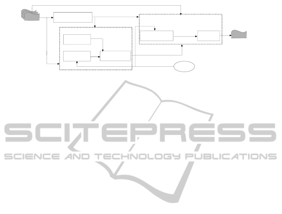
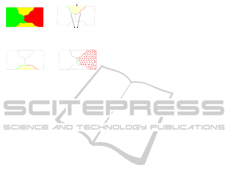
picture surface

selection

view interpolation

Novel Perspective Synthesis

structure from motion

user efforts

manual perspective

specification

input images

multi-perspectives

panorama

camera pose and

3D points

Panorama Generation

synthesized perspectives

perspective

composition

perspective

configuration

dense stereo

3D geometrical

information

original perspectives

Figure 1: The system framework.

misalignments. The framework consists of two steps:

ﬁrstly, parts of various perspectives are selected such

that visual discontinuities among those parts can be

minimized, and then, remaining artifacts are further

suppressed through a fusion process.

An overview of our system is presented in Fig 1.

In our system, street scenes are captured by a video

camera (with a ﬁxed intrinsic camera parameter K)

moving along the scene to capture it looking side-

ways. The camera pose of each input image (i.e.,

the translation vector T, the rotation matrix R and K)

is recovered using our Structure from Motion (SfM)

system, together with a sparse set of reconstructed 3D

scenes points. From recovered camera poses, novel

perspectives are synthesized based on 3D geometri-

cal information estimated using our dense stereo al-

gorithm. An interface for manually specifying the

multi-perspective conﬁguration is provided based on

our perspective composition framework, which com-

bines different perspectives (original or novel) to form

the resultant panorama.

The rest of this paper is organized as follows. Sec-

tion 2 presents background. Section 3 presents our al-

gorithm for synthesizing novel perspectives. Section

4 describes our perspective composition framework.

Results and discussions are presented in Section 5 and

Section 6 concludes this paper.

2 BACKGROUND

The earliest attempt at combining images captured

at different viewpoints is perhaps view interpolation,

which warps pixels from input images to a reference

coordinate using a pre-computed 3D scene geome-

try (Szeliski and Kang, 1995; Kumar et al., 1995;

Zheng and Kang, 2007). There are two main prob-

lems with these approaches: to establish an accurate

correspondence for stereo is still a hard vision prob-

lem, and there will likely be holes in the resultant im-

age due to sampling issues of the forward mapping

and the occlusion problem. Another thread is based

on optimal seam (Shum and Szeliski, 2000; Agarwala

et al., 2006), which stitches input images with their

own perspective and formulates the composition into

a labeling problem, i.e., pixel values are chosen to be

one of the input images. Results are inherently multi-

perspective. However, these approaches only work

well for roughly planar scene, as for scenes with large

depth variations, it is often impossible to ﬁnd an opti-

mal partition that can create seamless mosaics.

The strip mosaic offers a better alternative. The

basic idea is to cut a thin strip from a dense col-

lection of images and put them together to form a

panorama. In its early form, the push-broom model

(Zheng, 2003; Peleg et al., 2000), the resultant im-

age is parallel in one direction and perspective in

the other, while the crossed-slits (Zomet et al., 2003)

model is perspective in one direction and is perspec-

tive from a different viewpoint in the other direction.

Therefore, the aspect ratio distortion is inherent due

to the different projections along the two directions.

In addition, because scenes within each strip are

rendered from a regular pinhole perspective, given a

certain strip width, there is a depth at which scenes

show no distortion. For a further depth, scenes might

be duplicately rendered, i.e., over-sampled, while for

a closer depth, scenes cannot be fully covered, i.e.,

under-sampled. In the literature, this kind of artifact

is named a sampling error distortion (Zheng, 2003),

see Fig 2.

Unlike the view interpolation and optimal seam,

even for scenes with complex geometrical struc-

tures, strip mosaic can still produce visually accept-

able results in spite of the fore-mentioned aspect ra-

tio and sampling error distortions. Therefore, the

strip mosaic provides a foundation upon which multi-

perspective panoramas in a large scale can be con-

structed. An interactive approach is presented in (Ro-

man et al., 2004), where several perspectives in the

form of vertical slits are speciﬁed by users and gaps

in-between them are ﬁlled with inverse perspectives.

Some other approaches attempt to automatically de-

GRAPP 2012 - International Conference on Computer Graphics Theory and Applications

228

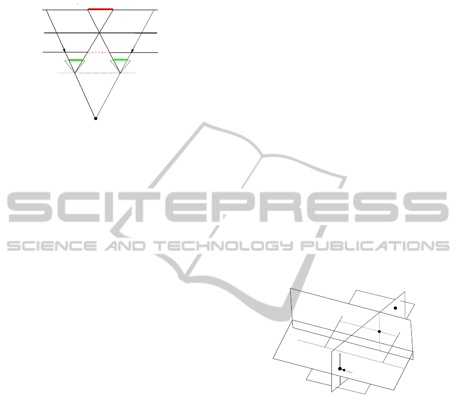
camera trajectory

vertical slit

strip width

under sampled

over sampled

non-distortion depth

Figure 2: The sampling error distortion is caused by the

depth parallax.

tect the multi-perspective conﬁguration through min-

imizing metrics for measuring undesired effects, e.g.,

the colour discrepancy between consecutive strips

(Wexler and Simakov, 2005) or the aspect ratio dis-

tortion (Roman and Lensch, 2006; Acha et al., 2008)

3 NOVEL PERSPECTIVE

SYNTHESIS

3.1 Single Direction View Interpolation

The novel perspective is rendered onto a 3D picture

surface, which is assumed to be perpendicular to the

ground plane of scenes. A working coordinate system

(WCS) is ﬁtted from camera poses of input sequence

to ensure that the ground plane is spanned by the X

and Z axes, so that the picture surface can be sim-

pliﬁed as a line in the top-down view of scenes, and

extruded along the up (Y) axis. Then input images are

rectiﬁed according to WCS.

The picture surface is deﬁned by a 3D plane π

and the X-Z plane of WCS is denoted as π

. If scenes

are exactly located on the picture surface, a point

(or pixel) of the resultant image p

= [x

]

can be

mapped to a point p = [x,y]

of the i

input image by

a projective transformation, i.e., the homography:

= H

= K[R

| t

(1)

where G is a 4×3 matrix that establishes the mapping

between a 2D point of the resultant image and a 3D

point X

= [X

]

on the picture surface, such

that:













= G











0 0 1











(2)

where V

and V

are vectors that parameterize X and

Y axes of the plane coordinate of the picture surface

and O is the origin of the plane coordinate. We choose

and V

as projections of the X and Y axes of WCS

onto the picture surface. s

and s

deﬁne the pixel

size along the X and Y axes of the image coordinate.

The choice of pixel size may affect the the rendering

effect, and the strategy for deﬁning a proper pixel size

is presented in Section 3.2.

If scenes do not lie exactly on the picture surface,

instead of using a uniform projective transformation,

a point from the input image should be individually

mapped onto the resultant image based on its actual

3D point X

. We assume that the (horizontal) projec-

tion center C

of a novel perspective always lies on

plane π

and the vertical slit L is the line that passes

through C

and perpendicular to π

, as shown in Fig 3.

The mapping from a point p = [x, y]

in the i

image

onto the picture surface is the intersection of 3 planes:

the picture surface π

, the plane π

that contains X

and the vertical slit L and the plane π

that contains

and the X axis of the i

camera that is centered at

, see Fig 3.

picture surface p

x-z plane p

camera trajectory

Figure 3: Points warping based on the 3D geometry.

Once the intersection is recovered, it is mapped to

the resultant image using G

, the pseudo-inverse of

G. This approach can be further simpliﬁed, since the

Y component of p

, i.e., y

, can be directly computed

using the homography H

. The value of the X com-

ponent x

depends on the actual 3D point. Suppose

that the picture surface π

intersects π

at a 3D line,

and X

are two points on that 3D line, then we

have:







((G

)

)((G

)

) − ((G

)

)((G

)

((G

)

)((G

)

) − ((G

)

)((G

)

((G

)

)((G

)

) − ((G

)

)((G

)



















= 0 (3)

where (G

)

denotes the k

row of the matrix G

With this equation, the value of x

can be solved from

the known value of y

. Since with one direction the

VISUALIZATION OF LONG SCENES FROM DENSE IMAGE SEQUENCES USING PERSPECTIVE COMPOSITION

229

mapping adopts the original projective transforma-

tion, and the other is based on the real 3D geometry,

this rendering strategy is named a “single direction

view interpolation” as opposed to the full perspective

interpolation.

picture surface p

x-z plane p

camera trajectory

resultant image

i-1

i+1

i-1

i+1

Figure 4: Rendering from a novel perspective. The pro-

jection center of the novel perspective is projected onto the

picture surface and then mapped to the ﬁnal resultant image.

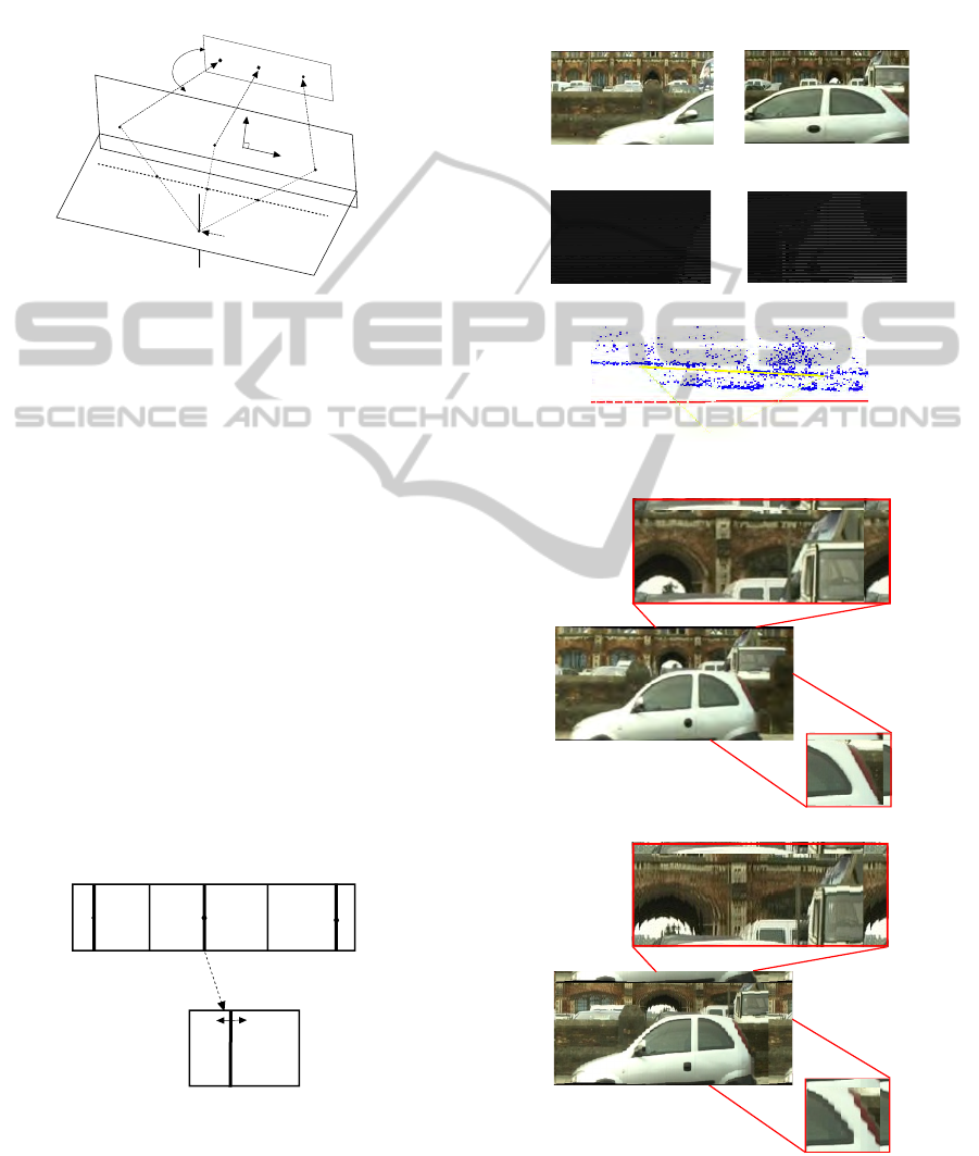
The point mapping is followed by the determi-

nation of which input image is selected to render a

point in the result. Such selection is inspired by the

the strip mosaic. We project each camera center C

onto a point in the resultant image c

along the line

connecting C

and the projection center of the novel

perspective C

, see Fig4. We deﬁne a vertical center

line CL

that passes c

on the resultant image. A ver-

tical split line BL

i,i+1

is drawn between any consecu-

tive camera center projections. The center line CL

then mapped to

in the corresponding input image

. We only examine pixels within a region around

. For each row of I

, we take the pixel on

the starting point and search on both sides. Once the

warped point onto the result is beyond the split line

i,i+1

or BL

i−1,i

, we proceed to the next row, see

Fig 5.

resultant image

i-1

i-1,i

i-1

i+1

i,i+1

i+1

Figure 5: Center lines and split lines on the resultant im-

age. Pixel warping is carried out within a region around the

center line mapping.

Fig 6(d) shows the result synthesized using our

single direction view interpolation. As compared to

that without the interpolation shown in Fig 6(e), the

sampling error distortion is removed. However, the

aspect ratio distortion still exists. For example, in Fig

6(d), the car in front of the middle low wall is appar-

ently squashed.

(a) Input images.

(b) Depth maps.

tion.

(d) Synthesized image with the interpolation.

(e) Synthesized image without the interpola-

tion.

Figure 6: A result of the novel perspective synthesis.

GRAPP 2012 - International Conference on Computer Graphics Theory and Applications

230

3.2 Rendering from Point Samples

Each projected point from an input image provides a

sample, and to render the resultant image is equivalent

to reconstructing a continuous function from these

scattered samples. This is done by convolving sam-

ples with a Gaussian ﬁlter. Then, a question naturally

arises as to what size of the pixel of the resultant im-

age is. The pixel size of the input image along the X

(horizontal) direction is known, i.e., s

. We compute

the average distance d

ave

of the picture surface devi-

ating from the camera trajectory. For simplicity, we

assume that the projection of the picture surface is a

straight line segment. In this case, the pixel size is

deﬁned as:

ave

(4)

where f is the focal length. The aspect ratio is chosen

as that of the input image, so the pixel size along the

Y (vertical) direction is: s

= αs

Unlike this uniform sampling strategy, another

choice is to use a non-uniform sampling, where the

pixel size varies according to the distance of the

picture surface deviating from the camera trajectory.

Given a point p on the picture surface, suppose that

the corresponding distance deviating from the camera

trajectory is represented by a function d(p), then the

pixel size at p is written as:

d(p)

(5)

The result shown in Fig 6 is rendered using the non-

uniform sampling strategy. Fig 7 compares results

rendered using uniform and non-uniform sampling

strategy.

Figure 7: Results of the non-uniform and uniform sampling

strategy. The result of the non-uniform sampling (middle),

and that of uniform sampling (bottom). The uniform sam-

pling strategy is aware of the shape of the picture surface,

while the result of the non-uniform sampling strategy more

agrees with human perception.

3.3 Dense Stereo

To estimate the depth (or, 3D geometry) map for each

point (pixel) in an image I

, a stereo process is per-

formed to I

and its neighboring image I

i+1

. The

stereo is accomplished in two steps: ﬁrstly, a corre-

spondence between I

and I

i+1

is detected, and then

the depth map is computed from the correspondence

together with camera poses of I

and I

i+1

To construct the correspondence, we adopt the

concept of the surface correspondence as suggested

in (Birchﬁeld and Tomasi, 1999). A surface can be

parameterized by the motion of its projections on I

and I

i+1

, such that: p + S(p) = p

. In this sense, the

correspondence detection is converted to determining

for each point p in I

which surface it should belong

to, and to calculating the motion parameter of that sur-

face. Since the stereo pair is assumed to be rectiﬁed

and the vertical movement is ignorable, the surface is

represented by a 1D afﬁne model:

S(p) =



∗ x + a

∗ y + b



(6)

We adopt a similar framework to that proposed in

(Birchﬁeld and Tomasi, 1999). The basic idea is to it-

eratively reﬁne the estimation by alternating between

two steps:

1. Given a labeled map of each point, we need to

ﬁnd the afﬁne motion parameter for each con-

nected segment. This is done by minimizing the

cost function

∑

p∈Ω

(p) − I

i+1

(p + S(p)))

, where

Ω denotes the set of all points in a segment. This

cost function is minimized using the the iterative

method proposed in (Shi and Tomasi, 1994).

2. Given a set of surfaces characterized by their

afﬁne motion parameters, each pixel is labeled as

belonging to one surface. The problem is solved

by a Markov Random Field (MRF) optimization

implemented using the Graph Cut algorithm (Kol-

mogorov and Zabih, 2004). The cost function of

the MRF consists of a data term that computes the

cost for a pixel p to be assigned with a surface

S(p), and a smooth term penalizing a pixel p and

its neighboring point q for having different sur-

face labels.

Fig 6(b) presents an example result of our dense

stereo algorithm.

4 PERSPECTIVE COMPOSITION

Our perspective composition framework consists of

two steps. Firstly, a decision must be made for each

VISUALIZATION OF LONG SCENES FROM DENSE IMAGE SEQUENCES USING PERSPECTIVE COMPOSITION

231

pixel of the resultant panorama as to which perspec-

tive should be adopted. Signiﬁcant pixel value dif-

ferences, and complex structures together with large

geometrical misalignments could make this labeling

process challenging and hence a sophisticated cost

function is proposed to take into account these vi-

tal factors. Visible discontinuities might still ex-

ist, which mainly occur along lines bordering adja-

cent segments rendered from different perspectives.

Therefore, in the second step, we suppress such dis-

continuities through blending information along these

boundary lines.

4.1 Perspective Selection

Given n perspectives: {V

}

n−1

, for each point p of

the resultant panorama, the perspectives selection is

represented by a labeling function: L(p) = i. Labels

of all points constitute a labeling conﬁguration: L,

the cost of which is formulated as a Markov Random

Field (MRF):

E(L) =

∑

(p,L(p)) +

∑

q∈N (p)

(p,q, L(p),L(q))

(7)

denotes the smooth term and E

denotes the data

term.

The smooth term E

consists of three terms: a

depth term, a colour term and a structure term, and the

measuring function is a weighted sum of these three

terms:

(p,q,L(p),L(q)) = E

d S

+ µ

c S

+ µ

g S

(8)

and µ

are weights.

Depth Smooth Term: The depth smooth term en-

courages the seam to go through regions where 3D

geometry coincides with the picture surface. We cal-

culate for each pixel of a perspective the residual er-

ror with respect to the picture surface. Each point

mapped from the input image onto the synthesized

image of a perspective constitutes a point sample.

Suppose that the point sample is extracted from the

input image I

, and let us denote the depth under the

camera coordinate of I

as d

(x). Then, we calculate

the depth of the corresponding point projected onto

the picture surface, denoted as d

). The residual

error of the point sample is:

) =











1.0 −

(x)

)

) ≥ d

(x)

1.0 −

)

(x)

) < d

(x)

(9)

The residual error of a grid point r

(p) of the i

perspective is computed by convolving these samples

with the Gaussian ﬁlter. Given a pair of neighbor-

ing pixels p and q of the resultant panorama, with as-

signed labels as L(p) and L(q), the depth smooth term

is:

d S

= r

L(p)

(p) + r

L(q)

L(p)

(q) + r

L(q)

(q)

(10)

Colour Smooth Term: To place the seam in re-

gions where pixel values from different perspectives

are similar, the colour smooth term is deﬁned as:

c S

∑

x∈W

| V

L(p)

(p + x) −V

L(q)

(p + x) |

∑

x∈W

| V

L(p)

(q + x) −V

L(q)

(q + x) |

(11)

where W is a window for the aggregation of differ-

ence, and N is the size of W.

Structural Smooth Term: To suppress structural

discontinuities, we deﬁne the structural smooth term

as (assuming the gradient ∇

captures the most struc-

tural information of an image):

g S

= | ∇V

L(p)

(p) − ∇V

L(q)

(p) |

+ | ∇V

L(p)

(q) − ∇V

L(q)

(q) |

(12)

The Data Term: A general form of the data term is

written as:

(p,L(p)) =



L(p)

(p) p ∈ V

L(p)

∞ p /∈ V

L(p)

(13)

L(p)

(p) measures the ﬁtness of a pixel to be assigned

with the label. We adopt a simple solution, i.e., use a

uniform function such that: U

L(p)

(p) ≡ 0.

4.2 Perspective Fusion

Discontinuities along the seam (or boundary line) be-

tween two segments rendered from different perspec-

tives need to be eliminated to produce a natural tran-

sition from one perspective to another, whilst, in the

meantime, we need to preserve original appearance as

much as possible. Here, we adopt a local method, i.e.,

information of one segment along the boundary line

is blended into the interior of the other one. Such in-

formation could simply be pixel values, and warping

vectors compensating for structural misalignments.

GRAPP 2012 - International Conference on Computer Graphics Theory and Applications

232

(a) Segments after the

pixel selection.

Self-Closure Boundary Line

Adjoinning Boundary Line

(b) Boundary fusion of

Ω

(d) Boundary fusion of

Ω

Figure 8: The boundary fusion in a monotonic order. The

order of involved perspectives is: L(0) < L(3) < L(1) =

L(2).

4.2.1 The Fusion Paradigm

Segments of each input perspective are extracted from

the result of the perspective selection. Let us assume

that there are m such segments, and for each seg-

ment k ∈ {0,..., m − 1}, the mapping function L(k)

denotes the index of the corresponding perspective i,

i ∈ {0,..., n − 1}. A segment Ω

is enclosed by its

boundary lines ∂Ω

. There are two kinds of boundary

lines: 1) adjoining boundary lines that are adjacent

to other segments, and 2) self-closure boundary lines

that do not border with any other segments, see Fig 8.

As for the former, information from other segments

need to be blended into the interior part of Ω

, whilst,

for the latter, we only consider information from Ω

itself.

We propose a monotonic fusion paradigm that

only performs the boundary fusion in a single direc-

tion. Let us suppose that two neighboring segments

Ω

and Ω

share a adjoining boundary line. With-

out losing generality, it is assumed that L( j) < L(k).

Information from Ω

along the boundary line are

blended into the interior part of Ω

, while, Ω

remains

unchanged. Fig 8 illustrates this monotonic fusion.

A proper order of input perspectives is needed.

We compute for each perspective the number of its

neighboring perspectives N(i), and then sort all input

perspectives with an ascending order of N(i). If two

perspectives have the same value of N(i), then the one

with more pixel number is placed before the other.

4.2.2 Blending of Pixel Values

To smoothly propagate pixel values of boundary lines,

the blending is constrained by the gradient ﬁeld of Ω

as suggested in (P

erez et al., 2003). Let the function

f (·) be the original pixel value at a certain pixel and

(·) denote the pixel value to be speculated in Ω

. In

addition, the function f

(·) denotes the pixel value at

the boundary line. The pixel value blending is casted

into a minimization problem, such that:

min

p∈Ω

| ∇ f

(p) − ∇ f (p) |

with f

(p) = f

(p) for p ∈ ∂Ω

(14)

According to the Euler-Lagrange theorem for

quadratic functions, such minimization can be con-

verted to a group of equations: ∆ f

(p) = div f (p) for

all p ∈ Ω

with f

(p) = f

(p) for p ∈ ∂Ω

, where

∆

denotes the second-order derivative and div f (·) is

the divergence. The second-order derivative can be

discretized using the Laplacian operator, yielding a

linear equation system, which is solved by our imple-

mentation of the multi-grid V-cycle algorithm special-

ized for irregular shaped segments.

4.2.3 Blending of Image Warping

Misalignments can be roughly grouped into two cat-

egories: a small structural misalignment, which is

usually brought by breaking edges along the adjoin-

ing boundary line, and a large structural misalign-

ment, which is mainly caused by signiﬁcant geomet-

rical misalignments. Fig 9(a) and 10(a) presents real

examples of these two types of misalignments. We

introduce two corresponding algorithms based on im-

age warping. Our system enables these two optional

algorithms to be selected by users for a given adjoin-

ing boundary line.

Structure Re-alignment. It is a common practice

to compensate for small structural misalignments

through locally re-aligning deviated edges, e.g., (Fang

and Hart, 2004; Jia and Tang, 2008). In the following,

this strategy is termed as “structure re-alignment”.

For each input perspective, we detect salient edges

with sufﬁciently large magnitudes. Given two neigh-

boring segments Ω

and Ω

, it is assumed that L(j) <

L(k), and hence the boundary information from Ω

blended into Ω

. We match edges striding over the ad-

joining boundary line bordering these two segments.

We enforce a one-to-one mapping that minimizes the

sum of edge difference measuring three factors: the

edge direction similarity, geometrical distance and

pixel value similarity. For a pair of matched edges,

we calculate the backward warping vector. Then we

interpolate warping vectors for those non-edge points

on the adjoining boundary line between Ω

and Ω

Warping vectors are blended into the interior of Ω

VISUALIZATION OF LONG SCENES FROM DENSE IMAGE SEQUENCES USING PERSPECTIVE COMPOSITION

233

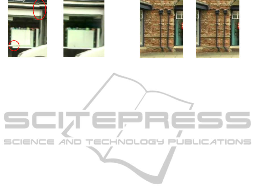
(a) A small structural

misalignment.

(b) After the structure

re-alignment.

Figure 9: A result of the structure re-alignment. In (a),

edges are broken by the seam. After the structure re-

alignment (b), edges are correctly aligned, and thus the

structural discontinuity is eliminated.

using the Poisson image editing (P

erez et al., 2003):

min

p∈Ω

| ∇z

(p) |

and for p ∈ ∂Ω

: z

(p) = z

(p),

where z

(p) denotes the warping vector to be spec-

ulated in Ω

and z

(p) is warping vector from the

boundary line.

Once the warping vector is calculated for each

pixel in Ω

, its pixel value of the warped image is

determined using bilinear interpolation. If there still

exists a large pixel value difference, we warp the gra-

dient ﬁeld of Ω

, and then, pixel value blending pre-

sented in the previous section is applied to the warped

gradient ﬁeld.

Segment Shift. To ﬁx the large structural misalign-

ment caused by the geometrical misalignment, the im-

age warping is based on a robust match between cor-

responding perspectives of the two adjacent segments.

The matching process is constrained by the geometri-

cal information. Firstly, a match region R is placed to

enclose the adjoining boundary line in V

L(k)

, and for

each pixel p in R, its corresponding depth informa-

tion is calculated from point samples for constructing

the perspective V

L(k)

through convolving such samples

with a Gaussian ﬁlter, and then it is re-projected onto

the perspective V

L( j)

as p

. The similarity between

p and p

is measured. The measurement is applied

to a patch centered at p (and p

) to allow for an off-

set. The one with the highest similarity degree is cho-

sen as the measuring result, and if it is above certain

threshold, then these two pixels are regarded as a cor-

rect match. A robust measuring function could be the

Normalized Cross-Correlation (NCC) performed over

a small window around a pixel. We also integrate into

our system the SIFT feature (Lowe, 2004), which is

reliable but sometimes too sparse.

Two matched pixels provide a backward warping

vector. For those pixels in R without robust matches,

(a) A large structural

misalignment.

(b) After the segment

shift.

Figure 10: A result of the segment shift. Due to the ge-

ometrical misalignment, a duplicate gutter is shown in (a),

after the segment shift, the ghost gutter is eliminated.

their warping vectors are estimated using known data.

In our system, we integrate two methods. If pixels

with known warping vectors are dense, a convolution

with a Gaussian ﬁlter is applied. On the other hand, if

such pixels are sparse (e.g., extracted from SIFT fea-

ture matching), a Radial Basis Function (RBF)-based

interpolation with thin-plate spline kernal (Wahba,

1990) is adopted.

Now, a warping vector is associated with each

pixel on the adjoining boundary between Ω

and Ω

These warping vectors are then blended into the in-

terior of Ω

using the poisson image editing as de-

scribed above. This strategy often induces a large

image deformation, which would cause parts of one

segments shifted towards the other, and therefore we

name it as “segment shift”.

5 RESULTS AND DISCUSSION

Experiments have been conducted on real urban

scenes. We demonstrate in Fig 11 how the perspective

composition can be used to create a multi-perspective

panorama from a manually speciﬁed perspective con-

ﬁguration. The perspective conﬁguration is shown

in Fig 11(d), which is mixed with both novel and

original perspectives. The original perspective is ren-

dered through mapping the corresponding input im-

age onto the picture surface using a projective trans-

form as deﬁned in 1. The novel perspective is syn-

thesized using our single direction view interpolation.

Fig 11(a) shows the result of the MRF optimization

for the perspective selection, where adjoining bound-

ary lines (seams) are highlighted. Fig 11(b) shows

the map of residual error with respect to the picture

surface, from which one can see that seams produced

by the MRF optimization are roughly placed in areas

with low residual errors. Fig 11(c) presents the ﬁnal

panorama after the boundary fusion. More results are

GRAPP 2012 - International Conference on Computer Graphics Theory and Applications

234

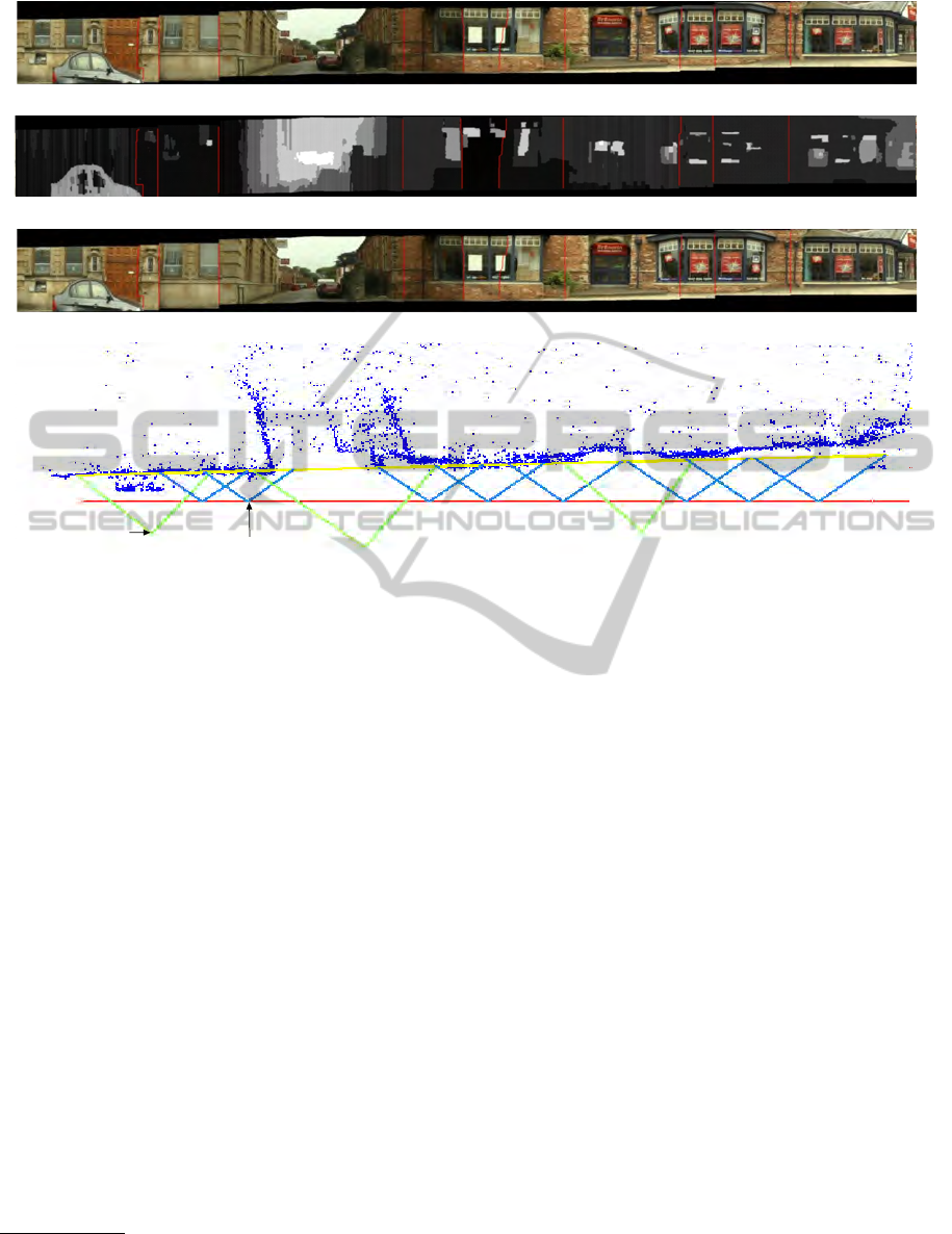
(a)

(b)

(c)

novel perspective

original perspective

(d)

Figure 11: A Panorama created from the perspective composition. In the multi-perspective conﬁguration (d), original per-

spectives are denoted as blue and novel ones are denoted as green. The result of MRF optimization is shown in (a) and the

composed residual error map is shown in (b). The ﬁnal panorama after boundary fusion is shown in (c).

shown in Fig 12. (Parts of fusion results are already

shown in Fig 9(b) and 10(b)).

We are not the ﬁrst to generate multi-perspective

panoramas through perspective composition. The ap-

proach presented in (Agarwala et al., 2006) takes orig-

inal perspectives as input, and use the MRF optimiza-

tion to select a perspective for rendering each pixel

in the resultant panorama. This approach works quite

well for mainly planar scenes. However, due to the

lack of facility to synthesize novel perspectives that

are wide enough to cover scenes not on the main plane

(picture surface), a seam placed at the area corre-

sponding to the off-plane scenes would induce serious

visual artifacts. Fig 13 presents an example result of

this approach, which is visually unacceptable

There are several existing approaches that address

the problem using synthesized novel perspectives.

However, they assume that input perspectives are pre-

cisely registered with each other, and therefore no fur-

ther composition processing is required in their sys-

tem. For example, the interactive approach described

in (Roman et al., 2004) only allows a set of disjoint

Actually, they use a ﬁsh-eye camera to expand the ﬁled

of view (FOV) of input images. However, the FOV of an

image is still limited.

perspectives to be speciﬁed, and these disjoint per-

spectives are simply connected by a set of inverse per-

spectives in between them. Obviously, their approach

restricts content that can be conveyed in the resultant

panorama, e.g., the perspective conﬁguration as pre-

sented in Fig 11(d) can never be achieved with their

approach.

6 CONCLUSIONS

This paper presents a system for producing multi-

perspective panoramas from dense video sequences.

Our system uses estimated 3D geometrical informa-

tion to eliminate the sampling error distortion in the

synthesized novel perspective. Then a perspective

composition framework is presented to combine dif-

ferent perspectives by suppressing their pixel value

and structural discrepancy. Compared to the exist-

ing methods, the perspective composition not only re-

moves noticeable artifacts, but also relieves some con-

straints imposed on the perspective conﬁguration that

a resultant panorama can be properly generated from.

The main problem of our approach is the aspect

ratio distortion associated with the synthesized novel

VISUALIZATION OF LONG SCENES FROM DENSE IMAGE SEQUENCES USING PERSPECTIVE COMPOSITION

235

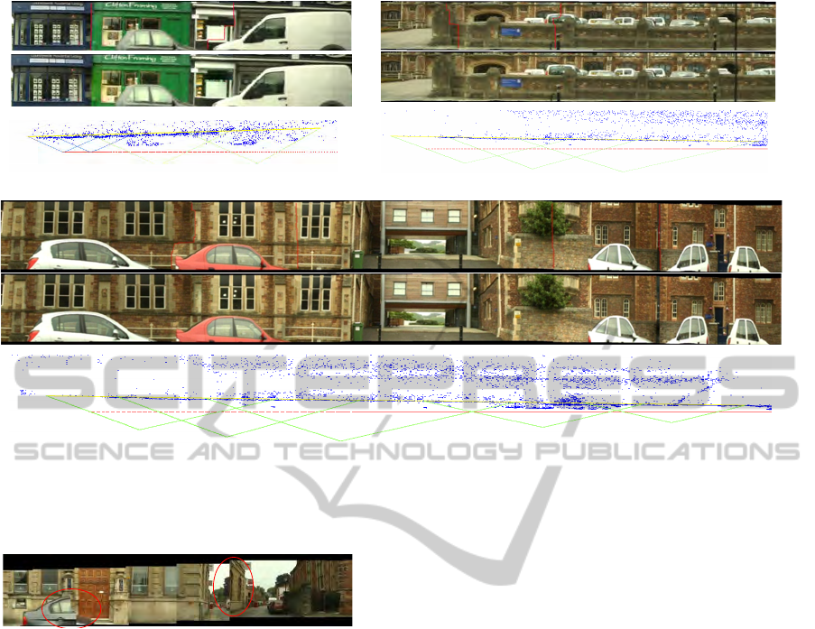
(a) (b)

(c)

Figure 12: Multi-perspective panoramas of urban scenes. For each result, the outcome of the MRF optimization (top) is

blended using our boundary fusion algorithm (middle).

Figure 13: A Panorama created from pure original perspec-

tives (Agarwala et al., 2006). Input image sequence is re-

sampled to get a set of sparse original perspectives, which

are combined using the MRF optimization. For scenes off

picture surface, visual artifacts are noticeable.

perspective. The cause of this problem lies in the fact

that we are lack of information along the direction

perpendicular to the direction of the camera move-

ment. In the future, we shall look into the use of an

array of cameras mounted on a pole to collect enough

information along the direction perpendicular to the

camera movement. Another interesting extension is

to introduce into our system some kinds of interac-

tive viewing facility, so that users can choose to view

scenes of interest at a high resolution or from a partic-

ular perspective such as the Street Slide system (Kopf

et al., 2010).

REFERENCES

Acha, A., Eagel, G., and Peleg, S. (2008). Minimal Aspect

Distortion (MAD) mosaicing of long scenes. Interna-

tional Journal of Computer Vision, 78(2-3):187–206.

Agarwala, A., Agrawala, M., Cohen, M., Salesin, D., and

Szeliski, R. (2006). Photographing long scenes with

multi-viewpoint panoramas. ACM Transactions on

Graphics, 25(3):853 – 861.

Birchﬁeld, S. and Tomasi, C. (1999). Multiway cut for

stereo and motion with slanted surfaces. In Proceed-

ings of the International Conference on Computer Vi-

sion, pages 489–495.

Brown, M. and Lowe, D. G. (2003). Recognising panora-

mas. In Proceedings of IEEE International Confer-

ence on Computer Vision, volume 2, pages 1218–

1225.

Fang, H. and Hart, J. C. (2004). Textureshop: texture syn-

thesis as a photograph editing tool. In Proceedings of

SIGGRAPH, volume 23, pages 354–359.

Jia, J. and Tang, C.-K. (2008). Image stitching using struc-

ture deformation. IEEE Transactions on Pattern Anal-

ysis and Machine Intelligence, 30(4):617–631.

Kolmogorov, V. and Zabih, R. (2004). What energy func-

tions can be minimized via graph cuts. IEEE Trans-

actions on Pattern Analysis and Machine Intelligence,

26(2):147–159.

Kopf, J., Chen, B., Szeliski, R., and Cohen, M. (2010).

Street slide: Browsing street level imagery. ACM

Transactions on Graphics, 29(4):96:1–96:8.

Kumar, R., Anandan, P., Irani, M., Bergen, J., and Hanna,

K. (1995). Representation of scenes from collections

of images. In Proceedings of IEEE Workshop on Rep-

resentation of Visual Scenes, pages 10–17.

GRAPP 2012 - International Conference on Computer Graphics Theory and Applications

236

Lowe, D. (2004). Distinctive image features from scale-

invariant keypoints. International Journal of Com-

puter Vision, 60(2):91–110.

Peleg, S., Rousso, B., Rav-Acha, A., and Zomet, A. (2000).

Mosaicing on adaptive manifold. IEEE Transac-

tions on Pattern Analysis and Machine Intelligence,

22(10):1144–1154.

erez, P., Gangnet, M., and Blake, A. (2003). Poisson

image editing. In Proceedings of SIGGRAPH, vol-

ume 22, pages 313–318.

Roman, A., Garg, G., and Levoy, M. (2004). Interactive

design of multi-perspective images for visualizing ur-

ban landscapes. In Proceedings of IEEE Visualization,

pages 537–544.

Roman, A. and Lensch, H. (2006). Automatic multiperspec-

tive images. In Proceedings of Eurographics Sympo-

sium on Rendering, pages 161–171.

Shi, J. and Tomasi, C. (1994). Good features to track.

In Proceedings of the IEEE Computer Society Con-

ference on Computer Vision and Pattern Recognition,

pages 593–600.

Shum, H. and Szeliski, R. (2000). Construction of

panoramic image mosaics with global and local align-

ment. International Journal of Computer Vision,

36(2):101–130.

Szeliski, R. and Kang, S. (1995). Direct methods for visual

scene reconstruction. In Proceedings of IEEE Work-

shop on Representation of Visual Scenes, pages 26–

33.

Szeliski, R. and Shum, H. (1997). Creating full view

panoramic image mosaics and environment maps.

Journal of Computer Graphics, 31:251–258.

Wahba, G. (1990). Spline Models for Observational Data.

SIAM.

Wexler, Y. and Simakov, D. (2005). Space-time scene man-

ifolds. In Proceedings of the International Conference

on Computer Vision, volume 1, pages 858 – 863.

Zheng, J. (2003). Digital route panoramas. IEEE Multime-

dia, 10(3):57– 67.

Zheng, K. C. and Kang, S. B. (2007). Layered depth panora-

mas. In Proceedings of the IEEE Computer Society

Conference on Computer Vision and Pattern Recogni-

tion, pages 1–8.

Zomet, A., Feldman, D., Peleg, S., and Weinshall, D.

(2003). Mosaicing new views: The crossed-slits pro-

jection. IEEE Transactions on Pattern Analysis and

Machine Intelligence, 25(6):741– 754.

VISUALIZATION OF LONG SCENES FROM DENSE IMAGE SEQUENCES USING PERSPECTIVE COMPOSITION

237