
GPU OPTIMIZATION AND PERFORMANCE ANALYSIS OF A
3D CURVE-SKELETON GENERATION ALGORITHM
J. Jiménez and J. Ruiz de Miras
Department of Computer Science, University of Jaén, Campus Las Lagunillas s/n, 23071 Jaén, Spain
Keywords: Curve-skeleton, 3D Thinning, CUDA, GPGPU, Optimizations, Fermi.
Abstract: The CUDA programming model allows the programmer to code algorithms for executing in a parallel way
on NVIDIA GPU devices. But achieving acceptable acceleration rates writing programs that scale to
thousands of independent threads is not always easy, especially when working with algorithms that have
high data-sharing or data-dependence requirements. This type of algorithms is very common in fields like
volume modelling or image analysis. In this paper we expose a comprehensive collection of optimizations
to be considered in any CUDA implementation, and show how we have applied them in practice in a
complex and not trivially parallelizable case study: a 3D curve-skeleton calculation algorithm. Two
different GPU architectures have been used to test the implications of each optimization, the NVIDIA
GT200 architecture and the new Fermi GF100. As a result, although the first direct CUDA implementation
of our algorithm ran even slower than its CPU version, overall speedups of 19x (GT200) and 68x (Fermi
GF100) were finally achieved.
1 INTRODUCTION
GPGPU (General-Purpose computing on Graphics
Processing Units) has undergone significant growth
in recent years due to the appearance of parallel
programming models like NVIDA CUDA (Compute
Unified Device Architecture) (NVIDIA A, 2011) or
OpenCL (Open Computing Language) (KHRONOS,
2010). These programming models allow the
programmer to use the GPU for resolving general
problems without knowing graphics. Thanks to the
large number of cores and processors present in
current GPUs, high speedup rates could be achieved.
But not all problems are ideal for parallelizing
and accelerating on a GPU. The problem must have
an intrinsic data-parallel nature. Data parallelism
appears when an algorithm can independently
execute the same instruction or function over a large
set of data. Data-parallel algorithms can achieve
impressive speedup values if the memory accesses /
compute operations ratio is low. If several memory
accesses are required to apply few and/or light
operations over the retrieved data, obtaining high
speedups is complicated, although it could be easier
with the automatic cache memory provided in the
new generation of NVIDIA GPUs. These algorithms
that need to consider a group of values in order to
operate over a single position of the dataset are
commonly known as data-sharing problems (Kong
et al., 2010). The case study of this paper, a 3D
thinning algorithm, belongs to this class of
algorithms and shares characteristics with many
other algorithms in the areas of volume modelling or
image analysis.
Some optimizations and strategies are explained
in vendor guides (NVIDIA A, 2011); (NVIDIA B,
2011), books (Kirk and Hwu, 2010); (Sanders and
Kandrot, 2010) and research papers (Huang et al.,
2008); (Ryoo et al., 2008); (Kong et al., 2010);
(Feinbure et al., 2011). In most cases, the examples
present in these publications are too simple, or are
perfectly suited to the characteristics of the GPU.
Furthermore, the evolution of the CUDA
architecture has meant that certain previous efforts
on optimizing algorithms are not completely
essential with the new Fermi architecture
(Wittenbrink et al., 2011). None of those studies can
assess the implications of the optimizations based on
the CUDA architecture used. Recent and interesting
works present studies in this respect, e.g. (Reyes and
de Sande, 2011); (Torres et al., 2011), but only loop
optimization techniques, in the first paper, and
simple matrix operations, in the second paper, are
discussed.
77
Jiménez J. and Ruiz de Miras J..
GPU OPTIMIZATION AND PERFORMANCE ANALYSIS OF A 3D CURVE-SKELETON GENERATION ALGORITHM.
DOI: 10.5220/0003852600770086
In Proceedings of the International Conference on Computer Graphics Theory and Applications (GRAPP-2012), pages 77-86
ISBN: 978-989-8565-02-0
Copyright
c
2012 SCITEPRESS (Science and Technology Publications, Lda.)

For GPGPU, Fermi architecture has a number of
improvements such as more cores, a higher number
of simultaneous threads per multiprocessor,
increased double-precision floating-point capability,
new features for C++ programming and error-
correcting code (ECC). But within the scope of data-
sharing and memory-bound algorithms, the most
important improvement of the Fermi architecture is
the existence of a real cache hierarchy.
In the rest of the paper, we firstly describe our
case study, a 3D thinning algorithm for curve-
skeleton calculation. Later we exposed our hardware
configuration and the voxelized models that we used
to check the performance of the algorithm. Next, we
analyze one by one the main optimizations for two
different CUDA architectures (GT200 and Fermi
GF100), and show how they work in practice.
Finally, we summarize our results and present our
conclusions.
2 CASE STUDY: A 3D THINNING
ALGORITHM
A curve-skeleton is a simple and compact 1D
representation of a 3D object that captures its
topological essence in a simple and very compact
way. Skeletons are widely used in multiple
applications like animation, medical image
registration, mesh repairing, virtual navigation or
surface reconstruction (Cornea et al., 2007).
Thinning is one of the techniques for calculating
curve-skeletons from voxelized 3D models.
Thinning algorithms are based on iteratively
eliminating those boundary voxels of the object that
are considered simple, e.g. those voxels that can be
eliminated without changing the topology of the
object. This process thins the object until no more
simple voxels can be removed. The main problem
that these thinning algorithms present is their very
high execution time, like any other curve-skeleton
generation technique. We therefore decided to
modify and adapt a widely used 3D thinning
algorithm presented by Palágyi and Kuba in (Palágyi
and Kuba, 1999) for executing on GPU in a parallel
and presumably more efficient way. Thus, all
previously exposed applications could benefit of that
improvement.
The 3D thinning algorithm presented in (Palágyi
and Kuba, 1999) is a 12-directional algorithm
formed by 12 sub-iterations, each of which has a
different deletion condition. This deletion condition
consists of comparing each border point (a voxel
belonging to the boundary of the object) and its
3x3x3 neighborhood (26-neighborhood) with a set
of 14 templates. If anyone matches, the voxel is
deleted; if not, the voxel remains. Each voxel
neighborhood is transformed by rotations and/or
reflections, which depend on the study direction,
thus changing the deletion condition.
In brief, the algorithm detects, for a direction d,
which voxels are border points. Next, the 26-
neighborhood of each border point is read,
transformed (depending on direction d) and
compared with the 14 templates. If at least one of
them matches, the border point is marked as
deletable (simple point). Finally, in the last step of
the sub-iteration all simple points are definitely
deleted. This process is repeated for each of the 12
directions until no voxel is deleted. The pseudo code
of the 3D thinning algorithm is shown in Figure 1,
where model represents the 3D voxelized object,
point is the ID of a voxel, d determines the direction
to consider, deleted counts the number of voxels
deleted in each general iteration, nbh and nbhT are
buffers used to store a neighborhood and its
transformation, and match is a boolean flag that
signals when a voxel is a simple point or not.
##START;
do{ //Iteration
deleted = 0;
for d=1 to d=12 { //12 sub-iterations
markBorderPoints(model, d);
for each BORDER_POINT do{
nbh =loadNeighborhood(model, point);
nbhT =transformNeighborhood(nbh, d);
match =matchesATemplate(nbhT);
if(match)
markSimplePoint(model, point);
}
for each SIMPLE_POINT do{
deletePoint(model, point);
deleted++;
}
}
}while(deleted>0);
##END;
Figure 1: Pseudo code of Palágyi and Kuba 3D thinning
algorithm. General procedure.
Regarding the functions, markBorderPoints()
labels as "BORDER_POINT", for the direction d, all
voxels which are border points, markSimplePoint()
labels the voxel point as "SIMPLE_POINT", and
deletePoint() deletes the voxel identified by point.
This algorithm has an intrinsic parallel nature,
GRAPP 2012 - International Conference on Computer Graphics Theory and Applications
78
Table 1: GPU specifications (MP: Multiprocessor, SP: Scalar Processor).
GPU Architecture
Computing
Capability
Number of
MPs
Number of
SPs
Thread Slots per MP Warp Slots per MP Block Slots per MP
GTX295
GT200 1.3 30 240 1024 32 8
GTX580
GF100 2.0 16 512 1536 48 8
GPU Max. Block Size Warp Size
Global
Memory
Constant
Memory
Shared Memory per
MP
L1 Cache
32-bit registers per
MP
GTX295
512 32 895 MB 64 KB 16 KB 0 16K
GTX580
1024 32 1472 MB 64 KB 48 KB/16KB 16KB/48KB 32K
because a set of processes are applied on multiple
data (voxels of the 3D object) in the same way. But
this is not fully parallelizable, since each sub-
iteration (one for each direction) strictly depends on
the result of the previous one and some CPU
synchronization points will be needed to ensure a
valid final result. In fact, we are dealing with a data-
sharing algorithm, where processing a data-item (a
voxel) needs to access other data-items (neighbors
voxels). Therefore kernel functions will have to
share data between them. This is a memory-bound
algorithm with a high ratio of slow global memory
reads to operations with this read data, and it is not
favourable in CUDA implementations. In addition,
these operations are very simple (conditional
sentences and Boolean checks), so it is difficult to
hide memory access latencies.
3 HARDWARE, 3D MODELS AND
FINAL RESULTS
Two different GPUs, based on GT200 and GF100
CUDA architectures, have been used to test and
measure the performance of our algorithm. The main
specifications of these GPUs are exposed in Table 1.
The GTX295 is installed on a PC with an Intel Core
i7-920 @ 2.67GHz 64-bits and 12 GB of RAM
memory (Machine A). The GTX580 is installed on a
server with two Intel Xeon E5620 @ 2.40GHz 64-
bits and 12 GB of RAM memory (Machine B). The
GTX580 has two modes: (1) Set preference to L1
cache use (48 KB for L1 cache and 16 KB for shared
memory), or (2) set preference to shared memory
(16 KB for L1 cache and 48 KB for shared
memory). We differentiate along this paper between
these modes when testing our algorithm.
Regarding the models used to test the CUDA
algorithm, we use a set of five 3D voxelized objects
with different complexity, features and sizes. These
models are: the Happy Buddha and Bunny models
from the Stanford 3D Scanning Repository (Stanford
University, 2011), Female pelvis and Knot rings
obtained in (SHAPES, 2011), and Nefertiti from
(VIA, 2011). All values of speedup, time or other
measures shown in this paper are the average value
for these five 3D models.
As an example, Figure 2 shows the Happy
Buddha model and its curve-skeleton calculated at a
high resolution of 512 x 512 x 512 voxels.
Figure 2: Stanford's Happy Buddha voxelized model and
its calculated 3D curve-skeleton.
Table 2 summarizes the main data obtained when
executing the 3D thinning algorithm. Time is
represented in seconds. As could be seen, the
improvement when executing on the GPU is
impressive. By analyzing the data, when the
algorithm runs on the CPU, running time directly
depends on the number of iterations. However, when
executing on GPU, this fact is not true, e.g. "Knot
Rings" model is more time consuming than "Happy
Buddha" model, although it implies less iterations.
Thus, we conclude that the GPU algorithm is more
sensitive to the irregularities and the topology of the
model.
In the next section we expose step by step the
strategies and their practical implications that we
have followed to achieve the optimal results showed
in Table 2 with our CUDA implementation of the
3D thinning algorithm. It is important to remark that
the single-thread CPU version of the thinning
algorithm is the one provided by its authors.
GPU OPTIMIZATION AND PERFORMANCE ANALYSIS OF A 3D CURVE-SKELETON GENERATION
ALGORITHM
79
Table 2: Main data and final execution results for the test
models at a resolution of 512 x 512 x 512. GTX580 in
shared memory preference mode.
Model Buddha Bunny Pelvis
Knot
Rings
Nefert.
Initial
Voxels
5,269,400
2
0,669,80
4
4,942,014
1
9,494,91
2
1
1,205,57
4
Final
Voxels
4,322 7,088 9,884 12,309 858
Iterations 65 125 102 59 53
MACHINE A - CPU i7-920 + GT200
CPU Time
(s)
351.30 676.09 552.66 332.58 288.32
GTX295
Time (s)
14.15 37.24 28.591 24.43 12.83
24.83x 18.15x 19.33x 13.61x 22.47x
MACHINE B - CPU INTEL XEON + GF100
CPU Time
(s)
376.34 732.95 596.46 353.13 307.68
5.19 10.95 8.13 5.70 4.47
72.51x 66.93x 73.36x 61.95x 68.83x
4 OPTIMIZATION APPROACHES
4.1 Avoiding Memory Transfers
Input data must be initially transferred from CPU to
GPU (global memory) through the PCI Express bus
(Kirk and Hwu, 2010). This bus has a low
bandwidth when compared with the speed of the
kernel execution, so one fundamental aspect in
CUDA programming is to minimize these data
transfers (Feinbure et al., 2011). In our first naive
CUDA implementation of the thinning algorithm,
this fact was not taken into account, since some
functions were launched on the GPU device and
others on the CPU host, thus transferring several
data between host and device. Therefore, the results
of this first implementation are very poor, as could
be seen in Figure 5 ("Memory Transfers" speedup).
The processing time was even worse than that
obtained with the CPU version. This shows that
direct implementations of not trivially parallelizable
algorithms may initially disappoint the
programmer´s expectations regarding GPU
programming. This occurs regardless of the GPU
used, which means that optimizations are necessary
for this type of algorithms even when running on the
latest CUDA architecture.
In our case, as previously mentioned, several
intermediate functions, such as obtaining a
transformed neighborhood, were initially launched
on the CPU. Therefore we must move these CPU
operations to the GPU, by transforming them into
kernels. This way the memory transfer bottleneck is
avoided, achieving a relative speedup of up to 1.43x
on the GTX295. A speedup between 1.49x (L1
cache preference) and 1.58x (shared memory
preference) is achieved for the GTX580 (see "All
processes to GPU" speedup in Figure 5).
4.2 Kernel Unification and
Computational Complexity
In our case study, the first kernel marks whether
voxels are border points or not, so that the second
kernel can obtain and transform their neighborhoods.
The third kernel detects which voxels are simple
points, so the fourth kernel can delete them. The
computational requirements of each kernel are very
low (conditional sentences and a few basic
arithmetic operations), therefore, the delays when
reading from global memory cannot be completely
hidden. It seems clear that this kernel division (a
valid solution in a CPU scope) is not efficient and
prevents a good general acceleration value. So we
restructured the algorithm by unifying the first three
kernels in only one, thus generating a new general
kernel with an increased computational complexity,
thus hiding the latency in accessing global memory.
The kernel unification usually implies a higher
register pressure. We take this fact into account
later, when discussing the MP occupancy and
resources in section 4.5.
The practical result for the GTX295 is a speedup
increase of up to 5.52x over the previous CUDA
version. The cumulative speedup so far is up to
7.89x over the original CPU algorithm. Higher
speedup rates are achieved for the GTX580, due to
the minimization of global memory read/write
instructions and the automatic cache system. A
speedup of 18.3x over the previous version is
achieved, nearly 29x respect the CPU version (see
"Kernel Unification" speedup in Figure 5). For the
first time we have overcome the performance of the
original CPU algorithm for all our test models and
model sizes.
4.3 Constant Memory
Constant memory is a 64 KB (see Table 1) cached
read-only memory, both on GT200 and GF100
architectures, so it cannot be written from the
kernels. Therefore, constant memory is ideal for
storing data-items that remain unchanged along the
whole algorithm execution and are accessed many
GRAPP 2012 - International Conference on Computer Graphics Theory and Applications
80

times from the kernels (Sanders and Kandrot, 2010).
Also, as a new improvement incorporated on the
GF100 architecture, the static parameters of the
kernel are automatically stored in constant memory.
In our 3D thinning algorithm we store in constant
memory the offset values indicating the position of
the neighbours of each voxel. These values depend
on the dimension of the model and do not change
along the thread execution, so are ideal for constant
memory. These values are accessed while checking
if a voxel belongs to the 3D model boundary and
when operating over a border point to obtain its
neighbourhood. Thus, global memory bandwidth is
freed. Our tests indicate that the algorithm is 11% to
18% faster, depending on the model size and the
GPU used, when using constant memory (see
“Constant Memory Usage” speedup in Figure 5).
4.4 Shared Memory Usage
Avoiding memory transfers between devices and
hiding the access memory latency time are important
factors in improving CUDA algorithms, whatever
GPU architecture, as outlined in sections 4.1 and
4.2. But focusing only on the GT200 architecture,
the fundamental optimization strategy is, according
to our experience, to use the CUDA memory
hierarchy properly. This is mainly achieved by using
shared memory instead of global memory where
possible (NVIDIA A, 2011); (Kirk and Hwu, 2010);
(Feinbure et al., 2011). However, the use of shared
memory on the newest GF100 GPUs may not be so
important, as would be seen later.
Shared memory is a fast on-chip memory widely
used to share data between threads within the same
thread-block (Ryoo et al., 2008). It can also be used
as a manual cache for global memory data by storing
values that are repeatedly used by thread-blocks. We
will see that this last use is not so important when
working on GF100-based GPUs, since the GF100
architecture provides a real cache hierarchy.
Shared memory is a very limited resource (see
Table1). It could be dynamically allocated during
the kernel launch, but not during the kernel
execution. This fact avoids that each thread within a
thread-block could allocate the exact amount of
memory that it needs. Therefore, it is necessary to
allocate memory to all the threads within a thread-
block, although not all of these threads will use this
memory. Several memory positions are wasted in
this case.
Based on our experience we recommend the
following steps for an optimal use of shared
memory: A) identify the data that are reused (data-
sharing case) or accessed repeatedly (cache-system
case) by some threads, B) calculate how much
shared memory is required, globally (data-sharing
case) or by each individual thread (cache-system
case), and C) deter-mine the number of threads per
block that maximizes the MP occupancy (more in
section 4.5).
Focusing now on our case study, the
neighborhood of each voxel is accessed repeatedly
so it can be stored in shared memory to achieve a
fast access to it. This way, each thread needs to
allocate 1 byte per neighbour. This amount of
allocated shared memory and the selected number of
threads per thread-block determine the total amount
of shared memory that each thread-block allocates.
We have tested our 3D thinning algorithm by
first storing each 26-neighborhood in global memory
and then storing it in shared memory. Testing on the
GTX295 with our five test models, a relative
speedup of more than 2x when using shared memory
is achieved. On the contrary, for the GTX580, the
relative speedup is minimal, achieving only a poor
acceleration of around 10%, with shared memory
preference mode. This indicates that the Fermi’s
automatic cache system works fine in our case. In
other algorithms, e.g. those in which not many
repeated and consecutive memory accesses are
performed, a better speedup could be obtained by
implementing a hand-managed cache instead of
using a hardware-managed one. If the L1 cache
preference mode is selected, using shared memory
decreases the performance on a 25%, because less
shared memory space is available. Despite this fact,
the use of shared memory is still interesting because
it releases global memory space, since the
neighbourhood could be directly transformed in
shared memory without modifying the original
model, which permits us to apply new improvements
later.
The overall improvement of the algorithm, up to
13.94x on GTX295 and 36.17x on GTX580, is
shown in Figure 5 (see “Shared Memory Usage”
speedup).
4.5 MP Occupancy
Once the required amount of shared memory is
defined, the number of threads per block that
generates the better performance has to be set. The
term MP occupancy refers to the degree of
utilization of each device multiprocessor. It is
limited by several factors. Occupancy is usually
obtained as:
GPU OPTIMIZATION AND PERFORMANCE ANALYSIS OF A 3D CURVE-SKELETON GENERATION
ALGORITHM
81

This estimation is the ratio of the number of active
warps per multiprocessor to the maximum number
of active warps. In this expression, empty threads
generated to complete the warp when the block size
is not a multiple of the warp size are considered as
processing threads. We calculate MP occupancy
based on the total resident threads as follows:
This expression offers a most reliable value of the
real thread slot percentage used to process the data.
We have considered both expressions in our analysis
for the sake of a more detailed study. It is important
to note that if the block size is a multiple of the warp
size both expressions return the same value. With
respect the parameters, BlockSize represents the
selected number of threads per thread-block. The
WarpSize parameter is the number of threads which
forms a warp, MaxMPThreads and MaxMPWarps is
the maximum number of threads and warps,
respectively, which a MP can simultaneously
manage, and ResidentBlocks represents the number
of blocks that simultaneously reside in an MP. We
can obtain this last value as:
MaxMPBlocks represents the maximum number of
thread-blocks that can simultaneously reside in each
MP. All these static parameters are listed in Table 1.
Obviously, if MaxMPThreads/WarpSize is equal to
WarpSize (like for the GTX295), the second
mathematical expression of ResidentBlocks is not
necessary.
But the block size is not the only factor that
could affect the occupancy value. Each kernel uses
some MP resources as registers or shared memory
(see previous section), and these resources are
limited (Ryoo, 2008) (Kirk and Hwu, 2010).
Obviously, an MP occupancy of 1 (100%) is always
desired, but sometimes it is preferable to lose
occupancy if we want to take advantage of these
other GPU resources.
Focusing now on registers, each MP has a limit
of 16 K registers (on 1.x devices) or 32 K registers
(on 2.x devices). Therefore, if we want to obtain a
full occupancy then each thread can use up to 16
registers (16 K / 1024 = 16 registers). On the other
hand, on the GTX580 each thread can use up to 21
registers (32 K / 1536 = 21.333 registers). Taking
this into account, we calculate the number of
simultaneous MP resident blocks in a more realistic
way as follows:
Where TotalSM represents the total amount of
shared memory per MP; RequiredSM is the amount
of shared memory allocated in each thread-block;
MaxThreadReg is the number of MP registers; and
RequiredReg is the number of registers that each
thread within a block needs.
In summary, there are three factors limiting the
MP occupancy: (1) the size of each thread-block, (2)
the required shared memory per block, and (3) the
number of registers used per thread. It is therefore
necessary to analyze carefully the configuration
which maximizes the occupancy. To check the exact
amount of shared memory and registers used by
blocks and threads, we can use the CUDA Compute
Visual Profiler (CVP) tool (NVIDIA C, 2011), or we
can set the '--ptxas-options=-v' option in the CUDA
compiler. CVP also directly reports the MP
occupancy value as the expression called
Occupancy_W in this paper.
In our case study, when compiling for devices
with a compute capability of 1.x, our threads never
individually surpass 16 used registers (the highest
value if we want to maximize occupancy on the
GTX295), so this factor is obviated when calculating
the number of resident bocks for this device. But
when compiling the same kernel for 2.x devices,
each thread needs 24 registers. This is because these
devices use general-purpose registers for addresses,
while 1.x devices have dedicated address registers
for load and store instructions. Therefore, registers
will be a limit factor when working on the GTX580
GPU.
If the block size increases, the required shared
memory grows linearly because allocated shared
memory depends directly on the number of threads
launched. However, the MP occupancy varies
irregularly when block size increases, as shown in
Figure 3 and Figure 4. Occupancy_W is always
equal or greater than Occupancy_T because
Occupancy_W gives equal weight to empty threads
and real processing threads. However, Occupancy_T
GRAPP 2012 - International Conference on Computer Graphics Theory and Applications
82
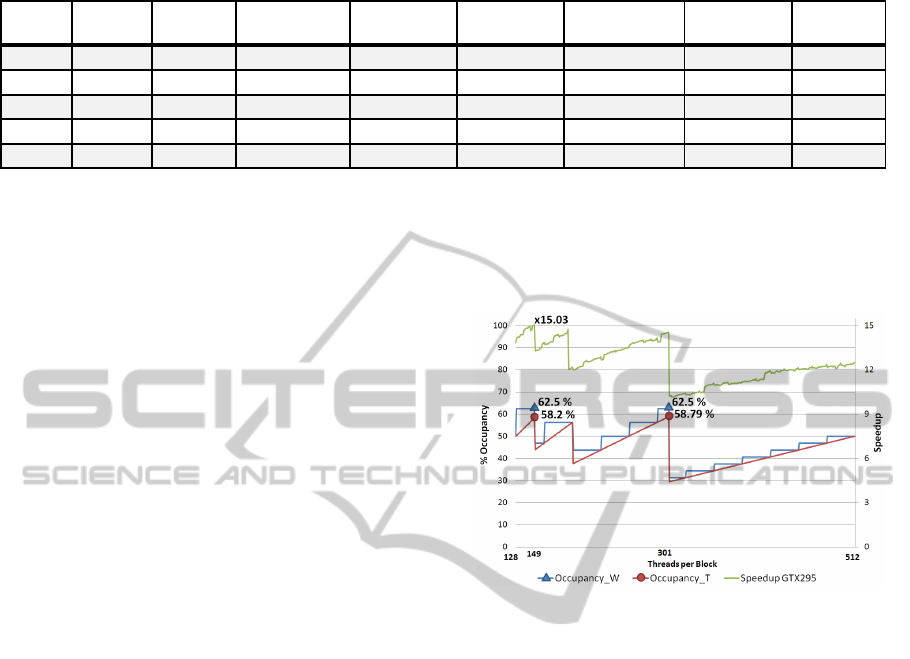
Table 3: Block size and speedup relationship on the GTX295. Average values for the five test models.
Block
Size
Thread
Slots
Warp
Slots
Warp Multiple Occupancy_T
Divergent
Branch
Overall
Throughput
Serialized
Warps
Speedup
128 512 16 Yes 50 %
3.67 %
1.328 GB/s
20,932
13.82x
149 596 20 No 58.20 % 3.75 %
2.198 GB/s
23,106
15.03x
288 576 18 Yes 56.25 % 3.89 % 1.350 GB/s 25,074 14.15x
301 602 20 No
58.79 %
3.77 % 2.017 GB/s 27,758 14.56x
302 302 10 No 29.49 % 3.79 % 1.231 GB/s 30,644 10.24x
only considers those threads that really work on the
3D model.
In brief, the amount of shared memory and the
number of required registers determine the resident
blocks, this number of blocks and the block size
determine how many warps and threads are
simultaneously executed in each MP, and the
occupancy is then obtained.
Focusing on the algorithm running on the
GTX295, the MP occupancy is maximized (62.5%)
when a value of 301 threads per block is set. A block
size of 149 obtains equal Occupancy_W percentage,
but 301 threads per block configuration also
maximizes Occupancy_T (58.79%). It seems clear
that one extra thread in a block could be a very
important factor. In our example, if we select 302
threads instead of 301, occupancy is reduced from
58.79% to 29.49%, which generates a reduction of
the algorithm´s performance. In the literature this is
sometimes called a performance cliff (Kirk and
Hwu, 2010), because a slight increase in resource
usage can degenerate into a huge reduction in
performance.
The highest occupancy is no guaranty for
obtaining the best overall performance. Therefore,
we perform an experimental test on the device for
determining exactly the best number of threads per
block for our algorithm. The analysis of the MP
occupancy factor obtains a set of values that would
lead to a good performance for our kernel execution.
But if we want to maximize the speedup it is
necessary to take into account other parameters.
Table 3 shows, for different block sizes, the values
obtained for the main parameters to be considered
on the GTX295 GPU. In this table, Divergent
Branch represents the percentage of points of
divergence with respect to the total amount of
branches (the lower the better). Overall Throughput
is computed as (total bytes read + total bytes written)
/ (GPU time) and refers to the overall global
memory access throughput in GB/s (the higher the
better).
The value Serialized Warps counts the number of
warps that are serialized because an address conflict
occurs when accessing to either shared memory or
constant memory (the lower the better). All these
parameters are obtained with the CVP (NVIDIA C,
2010).
Figure 3: Analysis of GTX295 MP Occupancy and the
speedup achieved with different "threads per block"
values. Average values for the five test models.
Table 3 also shows that the highest speedup is
achieved with a configuration of 149 threads per
block. Although that row does not have the highest
occupancy value, it has a low number of Serialized
Warps and also the highest memory throughput
value. It is important to note that the achieved
speedups are directly related to its corresponding
memory throughput. This fact indicates that the
algorithm is clearly memory bound, as previously
mentioned. The best values of Divergent Branch and
Serialized Warps appear with a size of 128 threads,
but its low occupancy and throughput prevent its
achieving a maximum speedup.
A very similar reasoning could be done by
analyzing for the GTX580 with the shared memory
preference mode. In Figure 4 are represented the
theoretical Occupancy_T and Occupancy_W trends.
According to our theoretical occupancy
calculations, a block-size of 192 threads, which is a
warp-size multiple, seems to be the better
configuration, achieving an 87.5% of Occupancy_T
and Occupancy_W. In fact, the best speedup is
achieved with this last value. By selecting the L1
GPU OPTIMIZATION AND PERFORMANCE ANALYSIS OF A 3D CURVE-SKELETON GENERATION
ALGORITHM
83
cache preference mode, we realize another
equivalent analysis, concluding that for this case 631
threads per block is the ideal value.
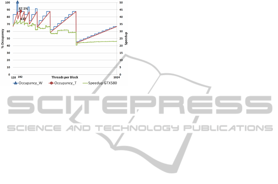
Figure 4: Analysis of GTX580 MP Occupancy and the
speedup achieved with different "threads per block"
values. Average values for the five test models.
Figure 3 and Figure 4 also shows the evolution
of the speedup when selecting different block sizes.
These lines follow the same trend as the
Occupancy_T line, especially in Figure 3,
demonstrating that this is a good parameter to take
into account when setting the thread-block size. The
irregularities of the speedup line are due to the
influence of the other parameters shown in Table 3.
Finally, “Block Size (Occupancy)” value in
Figure 5 represents the achieved speedup when we
select: 149 threads per block instead of 128 for the
GTX295, 192 threads per block instead of 149 for
the GTX580 in shared memory preference mode,
and 631 threads per block instead of 149 for the
GTX 580 in L1 cache preference mode.
4.6 Device Memory. Buffers
At this moment of the programming process we
have two kernels in our parallel CUDA algorithm:
the first kernel determines which voxels are simple
points and labels them, and the second one deletes
all simple points, so we are performing some extra
and inefficient writes to global memory. If the first
kernel directly delete simple points, the final result
would not be right because each kernel requires the
original value of its neighbors. We can duplicate the
structure which represents the 3D voxelized model
taking advantage of the high amount of global
memory present in GPU devices. Therefore, at this
time we also beneficiates of the use of shared
memory on both GPUs, since more global memory
is released. In this way, a double-buffer technique is
implemented and only one kernel must be launched.
This kernel directly deletes simple points by
reading the neighborhood from the front-buffer and
writing the result in the back-buffer. This ensures a
valid final result and, according to our tests,
improves the algorithm´s performance. This
improvement is greater if the voxelized 3D object
has a high number of voxels. In the case of our 3D
models, this optimization achieves an average
improvement of 25% on the GTX295, and an
acceleration of 52% and 83%, depending on the
selected mode, on the GTX580 (see “Double Buffer”
speedup in Figure 5).
4.7 Other Strategies
There are other optimization strategies that could
improve our parallel algorithm. One of them is to
avoid that threads within the same warp follow
different execution paths (divergence).
Unfortunately, in our case study it is very difficult to
ensure this because the processing of a voxel by a
thread depends directly on whether the voxel is a
border point or not, whether it is a simple point or
not, or if the voxel belongs to the object or not.
However, empty points and object points managed
by a warp are consecutive except when in-out or out-
in transition regarding the object boundary occurs.
This implies that the problem of divergence does
not greatly affect our algorithm. In fact, as shown in
Table 3, the percentage of divergent branches is
quite low. However, it is interesting to try different
combinations with our conditional sentences to get
better speedup.
It is also recommended to apply the technique of
loop unrolling, thus avoiding some intermediate
calculations which decrease the MP performance
(Ryoo et al., 2008). Shared memory is physically
partitioned into some memory. To achieve a full
performance of shared memory, each thread within a
half-warp has to read data from a different bank, or
all these threads have to read data from the same
bank. If one of these two options is not satisfied then
a partition camping problem occurs that decreases
the performance (Price et al., 2010). By applying all
these enhancements, our algorithm obtains a final
speedup of up to 19.68x for the GTX295. For the
GTX580, with the L1 cache preference mode, a final
speedup of 50.78x is achieved. This GPU achieves a
high speedup of 68.8x with the shared memory
preference mode (see “Other Strategies” speedup in
Figure 5). It is important to know that both CPU and
GPU applications are compiled in 64-bit mode.
GRAPP 2012 - International Conference on Computer Graphics Theory and Applications
84
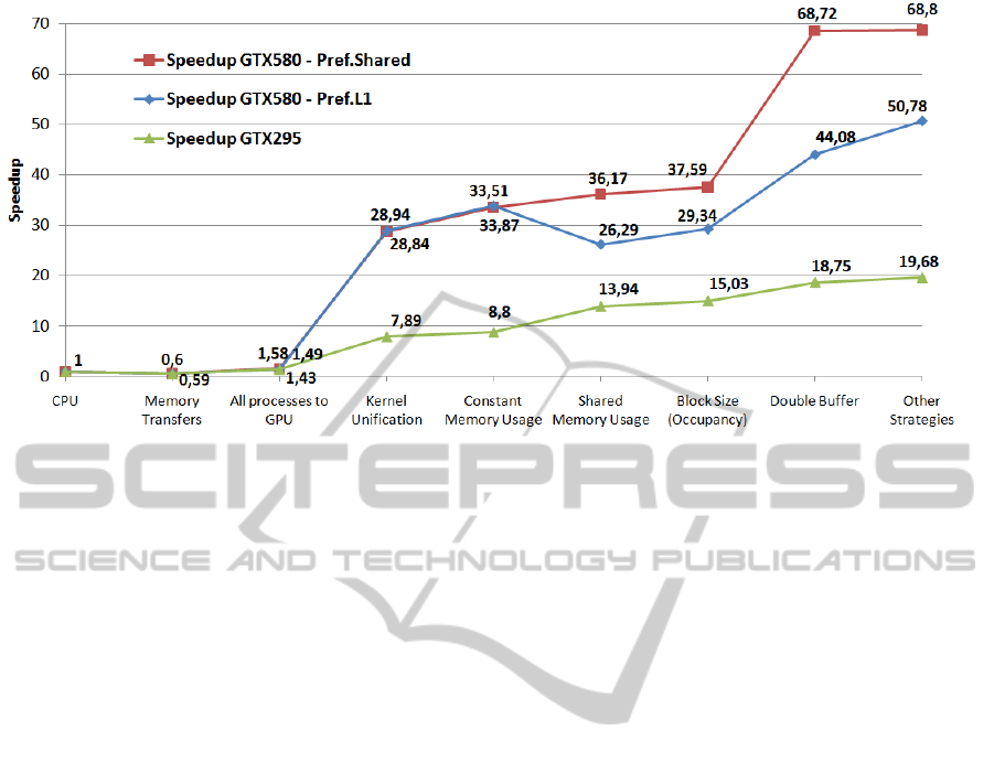
Figure 5: Summary of the main optimization strategies applied and their achieved speedups. Average values for the five test
models with size of 512 x 512 x 512.
5 CONCLUSIONS
We have detailed in a practical way the main CUDA
optimization strategies that allow achieving high
acceleration rates in a 3D thinning algorithm for
obtaining the curve-skeleton of a 3D model. Two
different GPU architectures have been used to test
the implications of each optimization, the NVIDIA
GT200 architecture and the new Fermi GF100.
Unlike typical CUDA programming guides, we have
faced to a real, complex and data-sharing problem
that shares characteristics with many algorithms in
the areas of volume modelling or image analysis.
We conclude that parallelizing a linear data-
sharing algorithm by using CUDA and achieving
high speedup values is not a trivial task. The first
fundamental task when optimizing parallel
algorithms is to redesign the algorithm to fit it to the
GPU device by minimizing memory transfers
between host and device, reducing synchronization
points and maximizing parallel thread execution.
Secondly, especially when working with GT200-
based GPUs, the programmer must have a deep
knowledge of the memory hierarchy of the GPU.
This allows the programmer to take advantage of the
fast shared memory and the cached constant
memory. Also, the hardware model must be taken
into account in order to maximize the processor´s
occupancy, the influence of divergent paths to the
thread execution, or which types of instructions have
to be avoided.
It has been demonstrated that the use of shared
memory as a manual cache may not be a
fundamental task (it depends on the algorithm
characteristics) with the new GF100 GPUs, due to
the presence of a new memory hierarchy and its
automatic cache system. Anyway, shared memory
still is a faster mechanism necessary to share data
between threads within a thread-block. The use of
shared memory also allows the programmer to
release global memory space, which can be used for
the implementation of other optimizations.
Obviously, if we decide to use shared memory in our
algorithm with the GF100 architecture, we must
select the shared memory preference mode to
achieve the highest speedup rate. The rest of
improvements exposed along this paper result in a
speedup increase in both GT200 and GF100 based
GPUs, so it is clear that the CUDA programmers
have to apply them even if they only work with the
latest Fermi GPUs.
We have shown the impressive speedup values
that our GF100 GPU achieves with respect to the
GT200. This is mainly due, in our case, to the high
number of cores, a higher amount of simultaneous
executing threads per MP, and the real cache L1 and
L2 hierarchy present on the GT100 architecture.
A summary of the main optimization strategies
detailed in this paper and their corresponding
average speedup rate are presented in Figure 5.
These results show that very good speedups can be
achieved in a data-sharing algorithm through the
particularized application of optimizations and the
reorganization of the original CPU algorithm.
GPU OPTIMIZATION AND PERFORMANCE ANALYSIS OF A 3D CURVE-SKELETON GENERATION
ALGORITHM
85

ACKNOWLEDGEMENTS
This work has been partially supported by the
University of Jaén, the Caja Rural de Jaén, the
Andalusian Government and the European Union
(via ERDF funds) through the research projects
UJA2009/13/04 and PI10-TIC-5807.
REFERENCES
Cornea, N. D., Silver, D., Min, P., 2007. Curve-skeleton
Properties, Applications and Algorithms. IEEE
Transactions on Visualization and Computer Graphics
13, 530-548.
Feinbure, F., Tröger, P., Polze, A., 2011. Joint Forces:
From Multithreaded Programming to GPU
Computing. IEEE Software.
Huang, Q., Huang, Z., Werstein, P., Purvis, M., 2008.
GPU as a General Purpose Computing Resource.
International Conference on Parallel and Distributed
Computing. Applications and Technologies. 151-158.
Kong J., Dimitrov M., Yang Y., Liyanage J., Cao L.,
Staples J., Mantor M., Zhou H., 2010. Accelerating
MATLAB Image Processing Toolbox Functions on
GPUs. Proceedings of the Third Workshop on
General-Purpose Computation on Graphics
Processing Units (GPGPU-3).
Kirk D. B., Hwu W. W., 2010. Programming Massively
Parallel Processors. Hands-on Approach. Morgan
Kaufmann Publishers.
Khronos OpenCL Working Group, 2010. The OpenCL
specification. V. 1.1. http://www.khronos.org/opencl/.
(A) NVIDIA, 2011. NVIDIA CUDA C Programming
Guide. V 4.0. http://developer.download.nvidia.com/
compute/DevZone/docs/html/C/doc/CUDA_C_Progra
mming_Guide.pdf
(B) NVIDIA, 2011. NVIDIA CUDA Best Practices Guide.
v 4.0. http://developer.download.nvidia.com/compu
te/DevZone/docs/html/C/doc/CUDA_C_Best_Practice
s_Guide.pdf
(C) NVIDIA, 2011. Compute Visual Profiler, User Guide.
http://developer.download.nvidia.com/compute/DevZo
ne/docs/html/C/doc/Compute_Visual_Profiler_User_
Guide.pdf
Price, D. K., Humphrey, J. R., Spagnoli, K. E., Paolini, A.
L., 2010. Analyzing the Impact of Data Movement on
GPU Computations. Proceedings of SPIE – The
International Society for Optical Engineering, 7705.
Palágyi, K., Kuba, A., 1999. A Parallel 3D 12-Subiteration
Thinning Algorithm. Graphical Models and Image
Processing 61, 199-221.
Reyes, R., De Sande, F., 2011. Optimize or wait? Using
llc fast-prototyping tool to evaluate CUDA
optimizations. Proceedings of 19th International
Euromicro Conference on Parallel, Distributed and
Network-Based Processing, 257-261.
Ryoo, S., Rodrigues, C. I., Baghsorkhi, S. S., Stone, S. S.,
Kirk, D. B., Hwu, W. W., 2008. Optimization
Principles and Application Performance Evaluation of
a Multithreaded GPU using CUDA. 13th ACM
SIGPLAN Symposium on Principles and Practice of
Parallel Programming.
Shape Repository, 2011. http://shapes.aimatshape.net/
Stanford University, 2011. The Stanford 3D Scanning
Repository. http://graphics.stanford.edu/data/3Dscan
rep/
Sanders, J., Kandrot, E., 2010. CUDA by Example. An
Introduction to General-Purpose GPU Programming,
Addison-Wesley.
Torres, Y., González-Escribano, A., Llanos, D. R., 2011.
Understanding the Impact of CUDA Tuning
Techniques for Fermi. Proceedings of the 2011
International Conference on High Performance
Computing and Simulation, HPCS 2011, art. no.
5999886, pp. 631-639.
VIA, 3D Repository, 2011. http://www.3dvia.com.
Wittenbrink, C. M., Kilgariff, E., Prabhu, A., 2011. Fermi
GF100 GPU Architecture. IEEE Micro 31, 50-59
GRAPP 2012 - International Conference on Computer Graphics Theory and Applications
86
