
A NEW REGION-BASED PDE FOR PERCEPTUAL IMAGE
RESTORATION
Baptiste Magnier, Philippe Montesinos and Daniel Diep
LGi2P de l’Ecole des Mines d’Al
`
es, Parc Scientifique Georges Besse, 30035 N
ˆ
ımes Cedex 1, France
Keywords:
Image Restoration, Rotating Filters, Edge Detection, Anisotropic Diffusion.
Abstract:
In this paper, we present a new image regularization method using a rotating smoothing filter. The novelty of
this approach resides in the mixing of ideas coming both from pixel classification which determines roughly
if a pixel belongs to a homogenous region or an edge and an anisotropic perceptual edge detector which
computes two precise diffusion directions. These directions are used by an anisotropic diffusion scheme.
This anisotropic diffusion is accurately controlled near edges and corners, while isotropic diffusion is applied
to smooth homogeneous and highly noisy regions. Our results and a comparison with anisotropic diffusion
methods applied on a real image show that our model is able to efficiently regularize images and to control the
diffusion.
1 INTRODUCTION
Partial Differential Equations (PDE’s) are widely
used in image restoration (Perona and Malik, 1990)
(Alvarez et al., 1992) (Weickert, 1998) (Tschumperl
´
e,
2006). Indeed, images are considered as evolving
functions of time and PDE’s enable to smooth the im-
age while preserving important structures or details
(Aubert and Kornprobst, 2006). Filtering techniques
like (Nagao and Matsuyama, 1979) (Tomasi and Man-
duchi, 1998) are not adapted to preserve small object
in presence of strong noise.
In (Perona and Malik, 1990) and (Black et al.,
1998), diffusion is isotropic on homogenous regions
but decreases and becomes anisotropic near bound-
aries. Diffusion control is done with finite differences
so that many contours of small objects or small struc-
tures are preserved. However, highly noisy images
may generate a lot of undesired artifacts.
Edge detection is often used to detect image
boundaries in order to control a diffusion process and
then to preserve contours present in the image in a
PDE scheme. The Mean Curvature motion method
(MCM) consists to diffuse only along the contour di-
rection (Catt
´
e et al., 1995), even in homogeneous re-
gions. In some diffusion approaches, Gaussian filter-
ing is used for gradient estimation, so the control of
the diffusion is more robust to noise (Alvarez et al.,
1992) (Weickert, 1998) (Tschumperl
´
e and Deriche,
2005) (Tschumperl
´
e, 2006). The intention is to rest-
rict the diffusion process only along the tangential di-
rection to the gradient near edges and to tune the dif-
fusion using the gradient magnitude. On regions con-
sidered as homogenous, the diffusion is isotropic, on
the contrary, at edge points, diffusion is anisotropic
and inhibited. Nevertheless, it remains difficult to
distinguish between high noise and small objects
that need to be preserved from the diffusion pro-
cess. In (Tschumperl
´
e, 2006), the author takes the
curvatures of specific integral curves into account
in the restoration process. PDE’s based on tensor
(Weickert, 1998) (Tschumperl
´
e and Deriche, 2005)
(Tschumperl
´
e, 2006) are very efficient on noise free-
images, but do not provide really homogeneous re-
gions when the noise is high, because the noise cre-
ates a fiber effect in the image. Indeed, these diffusion
methods are adapted for the preservation of thin struc-
tures in the image.
In this paper, we present a rotating filter (inspired
by (Montesinos and Magnier, 2010), (Magnier et al.,
2011c) and (Magnier et al., 2011b)) able to detect ho-
mogenous regions and edges regions, even in highly
noisy images. Then, we present an anisotropic edge
detector which defines two directions for pixels be-
longing to edges. Finally, we introduce a method
for anisotropic diffusion which controls accurately
the diffusion near edge and corner points and dif-
fuses isotropically inside noisy homogeneous regions.
In particular, our detector provides two different di-
rections on edge and corner points, these informa-
56
Magnier B., Montesinos P. and Diep D..
A NEW REGION-BASED PDE FOR PERCEPTUAL IMAGE RESTORATION.
DOI: 10.5220/0003853000560065
In Proceedings of the International Conference on Computer Vision Theory and Applications (VISAPP-2012), pages 56-65
ISBN: 978-989-8565-03-7
Copyright
c
2012 SCITEPRESS (Science and Technology Publications, Lda.)

tions enable an anisotropic diffusion in these direc-
tions contrary to (Alvarez et al., 1992) where only one
direction is considered. In (Magnier et al., 2011c), the
authors introduce a new diffusion method to remove
the textures. This approache diffuse in two differ-
ent directions of a contour for each pixel near edges.
However, they are not adapted for image restoration
because an efficient way of controlling the diffusion
is missing. In this paper, we extend this method to
restoration. More precisely, the diffusion is controlled
both by the gradient value and two directions issued
from an anisotropic edge detector (Montesinos and
Magnier, 2010).
We first present in section 2 our rotating smooth-
ing filter. A pixel classification using a bank of fil-
tered images is introduced in section 3. Thereafter,
we present a anisotropic edge detector based on half
smoothing kernels in section 4. Our anisotropic dif-
fusion scheme is introduced in section 5. Section
6 is devoted to experimental results and comparison
with other methods. Finally, section 7 concludes this
paper.
2 A ROTATING SMOOTHING
HALF FILTER
Y
X
1
2
_
1
2
_
(a) Smoothing filter.
θ
(b) Rotating
filters.
5 10 15 20 25 30
0
5
10
15
20
25
30
35
40
X axis
Y axis
(c) Discretized
filter.
Figure 1: A rotating smoothing half filter. For (c): µ = 10
and λ = 1.
In our method, for each pixel of the original image,
we use a rotating half smoothing filter (illustrated in
Fig. 1) in order to build a signal s which is a function
of a rotation angle θ and the underlying signal. As
shown in (Montesinos and Magnier, 2010), (Magnier
et al., 2011c) and (Magnier et al., 2011b), smoothing
with rotating filters means that the image is smoothed
with a bank of rotated anisotropic Gaussian half ker-
nels:
G
(µ,λ)
(x,y,θ) = C · I
θ
∗ H (−y) ·e
−
x
2
2λ
2
+
y
2
2µ
2
(1)
where I
θ
corresponds to a rotated image
1
of orienta-
tion θ, C is a normalization coefficient, (x,y) are pixel
coordinates, and (µ, λ) the standard-deviations of the
Gaussian filter. As we need only the causal part of the
filter, we simply “cut” the smoothing kernel by the
middle, this operation corresponds to the Heaviside
function H and the implementation is quite straight-
forward.
Some examples of smoothed images using our
half kernels G
(µ,λ)
(x,y,θ) are available in Fig. 2 (b)
and (c).
3 PIXEL CLASSIFICATION
In the following the image is represented as a function
defined as :
I(x,y) : R
2
→ R.
This case corresponds to grey level images.
3.1 Pixel Description
The application of the rotating filter at one point of an
image in a 360 scan, provides to each pixel a charac-
terizing signal. In the case of a gray level image, the
pixel signal is a single function s(θ) of the orientation
angle θ. Fig. 2(d) is an example of s-functions mea-
sured at 6 points located on a noisy image. Each plot
represents in polar coordinates the function s(θ) of a
particular point. From these pixel signals, we now
extract the descriptors that discriminate edges and re-
gions.
3.2 Flat Area Detection
The main idea for analyzing a 360 scan signal is to
detect significant flat areas, which correspond to ho-
mogeneous or noisy regions of the image. Fig. 3(a)
shows the pixel signal s(θ) extracted from a point be-
longing to a contour. After smoothing, the derivative
s
θ
(θ) is calculated and represented on Fig. 3(b). From
s
θ
(θ), flat areas are detected as intervals (i.e. angu-
lar sectors) with a small derivative (close to zero), i.e.
sets of values exceeding a given threshold s
th
in am-
plitude. Let us note α the largest angular sector. We
consider that we detect a flat area when 30 < α < 360
(degrees).
The noise removal method consists to diffuse
isotropically inside homogenous (point 3 of Fig. 2(a))
1
As explained in (Montesinos and Magnier, 2010), the
image is oriented instead of the filter because it increases
the algorithmic complexity and allows to use a recursive
Gaussian filter (Deriche, 1992).
A NEW REGION-BASED PDE FOR PERCEPTUAL IMAGE RESTORATION
57
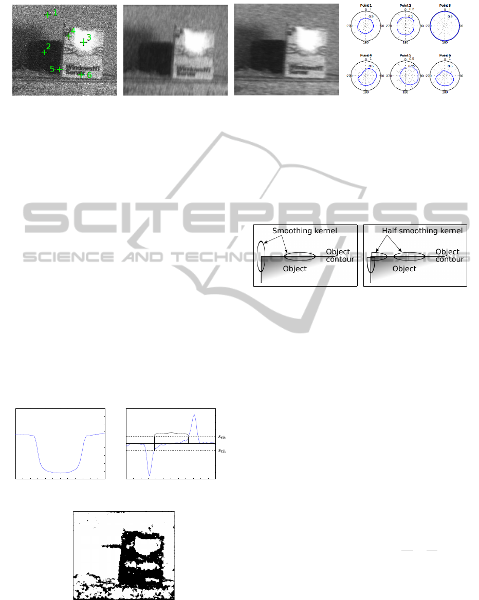
(a) Points selection in green
on a noisy image 420×395.
(b) Smoothed image θ = 10
degrees.
(c) Smoothed image θ = 275
degrees.
(d) Polar representation of s(θ)
for each points of (a).
Figure 2: Points selection and associated signal, µ = 10, λ = 1 and ∆θ = 5 (degrees).
and noisy regions (points 1 and 2) i.e. α = 360 (de-
grees). In order to keep sharp contours, the aim of this
approach is to diffuse anisotropically at edge points
(like points 5 and 6) and corner points (like point 4) so
as to preserve borders between regions. Black regions
in Fig. 3(c) show regions of flat areas have been de-
tected (30 < α < 360 in degrees) in the Fig. 2(a). So
this image will be smoothed anisotropically in black
regions of Fig. 3(c) and isotropically in white regions.
As shown in Fig. 3(c), flat area detection can be seen
as a rough edge detection method. In (Magnier et al.,
2011c), the curvatures of the signal s(θ) define two
directions used in anisotropic diffusion. These di-
rections are not enough precise for image restoration.
Here, we use the directions for the diffusion computed
from a new anisotropic edge detector which defines
also two directions, but much more precise, resulting
in a more precise diffusion.
0 30 60 90 120 150 180 210 240 270 300 330 360
0
0.05
0.1
0.15
0.2
0.25
0.3
0.35
0.4
0.45
s(θ)
degrees
0 30 60 90 120 150 180 210 240 270 300 330 360
−0.1
−0.08
−0.06
−0.04
−0.02
0
0.02
0.04
0.06
0.08
0.1
s
θ
(θ)
degrees
α
1
_
_
(a) Original signal s(θ). (b) First derivative of s(θ).
(c) Flat area regions in black.
Figure 3: Flat area detections from s(θ). µ = 10, λ = 1 and
∆θ = 5 (degrees).
4 EDGE DETECTION USING
HALF SMOOTHING KERNELS
(a) (b)
Figure 4: (a) Full and (b) Half Anisotropic Gaussian kernels
at linear portions of contours and at corners.
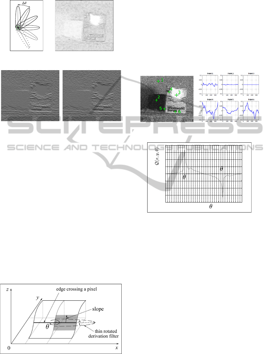
As diagrammed in Fig. 4 (a), steerable (Freeman
and Adelson, 1991) (Jacob and Unser, 2004) or
anisotropic edge detector (Perona, 1992) perform well
to detect large linear structures. However, near cor-
ners, the gradient magnitude decreases as the edge
information under the scope of the filter decreases.
Consequently, the robustness to noise decreases.
A simple solution to bypass this effect is to con-
sider paths crossing each pixel in several directions.
The idea developed in (Montesinos and Magnier,
2010) is to “cut” the derivative (and smoothing) ker-
nel in two parts: a first part along a first direction and
a second part along a second direction (see Fig. 4 (b).
At each pixel of coordinates (x, y), a derivation fil-
ter is applied to obtain a derivative information called
Q (x,y,θ):
Q (x,y,θ) = I
θ
∗C
1
· H (−y) ·x · e
−
x
2
2λ
2
+
y
2
2µ
2
(2)
where C
1
represents a normalization coefficient. As
diagrammed in Fig. 6, Q (x, y,θ) represents the slope
of a line issued from a pixel in the perpendicular di-
rection to this line (see Fig. 7(b) for several signals
Q (x,y,θ)) issued from several images derivatives (Fig
VISAPP 2012 - International Conference on Computer Vision Theory and Applications
58
+
+
+
+
+
+
_
_
_
_
_
_
(a) Rotated
derivation
filter.
(b) Gradient image.
(c) Image derivative at θ =
10
◦
.
(d) Image derivative at θ =
275
◦
.
Figure 5: Image in Fig. 2 (a) derivate using different orien-
tations with µ = 10 and λ = 1. Normalized images.
5). To obtain a gradient k∇Ik and its associated direc-
tion η on each pixel P, we first compute global ex-
trema of the function Q (x,y,θ), with θ
1
and θ
2
(as
illustrated in Fig. 7 (c)). θ
1
and θ
2
define a curve
crossing the pixel (an incoming and outgoing direc-
tion). Two of these global extrema can then be com-
bined to maximize k∇Ik, i.e. :
θ
1
= argmax
θ∈[0,360[
(Q (x,y,θ)), θ
2
= arg min
θ∈[0,360[
(Q (x,y,θ))
(3)
and k∇Ik = Q (x, y,θ
1
) −Q (x,y,θ
2
).
Once obtained k∇Ik, θ
1
and θ
2
, edges can easily
be extracted by computing local maxima of k∇Ik in
the direction of the angle (θ
1
+ θ
2
)/2 followed by an
hysteresis threshold (see (Montesinos and Magnier,
0
x
y
z
Figure 6: Estimation of the slope turning around a pixel.
The z axis represents the pixel intensity.
2010) for more details). In this paper, we are only
interested by the two directions (θ
1
,θ
2
) and the gradi-
ent magnitude used in our diffusion scheme in section
5.2.
Due to the lengths of the rotating filters, it enables
to keep a robustness agains noise and compute two
precise diffusion orientations in the directions of the
edges. In (Magnier et al., 2011a), the authors have
evaluated the edge detection used in this method as a
function of noise level.
(a) Points selection in
green on image in Fig.
1(d).
(b) Q (x,y,θ) for each points
of (a).
-0.04
-0.03
-0.02
-0.01
0
0.01
0.02
0.03
0.04
0
360
1
2
Discretized angle (degrees)
Quality function
l
l
l
90
180
270
l
(c) Extrema of a function Q (x, y,θ).
Figure 7: Points selection and its associated Q (x,y,θ),
µ = 10, λ = 1 and ∆θ = 2
o
.
5 ANISOTROPIC DIFFUSION IN
TWO DIRECTIONS WITH PDE
In several diffusion scheme: (Alvarez et al., 1992)
(Weickert, 1998) (Tschumperl
´
e and Deriche, 2005)
(Tschumperl
´
e, 2006), only one direction is predomi-
nantly considered at edges, corner points are treated
like edge points, this direction is tangential to the
edge. Tensor diffusion schemes preserve edges
(Weickert, 1998) (Tschumperl
´
e and Deriche, 2005)
(Tschumperl
´
e, 2006) but in order to remove high
noise while preserving contours, the standard devia-
tion of the Gaussian σ must be large. However this so-
lution will blur edges and break corners. For minimiz-
ing these effects we are going to consider the two di-
rections (θ
1
,θ
2
) provided by eq. 3 of the anisotropic
edge detector only in areas where flat areas have been
A NEW REGION-BASED PDE FOR PERCEPTUAL IMAGE RESTORATION
59
detected (Fig. 7(d)).
5.1 Diffusion Scheme in Two Directions
Unlike (Alvarez et al., 1992) (Weickert, 1998)
(Tschumperl
´
e and Deriche, 2005) (Tschumperl
´
e,
2006), our control function does not depend only
on the image gradient but on a pre-established clas-
sification map of the initial image. As stated in
section 3, this classification is a rough classifica-
tion between region and edges. Consequently, a dif-
fusion scheme with only this new control function
moves corner points according to the curvature of iso-
intensity lines. As a consequence, this scheme be-
haves as the MCM scheme (Catt
´
e et al., 1995), for
example a square is transformed into a circle after
some iterations. For minimizing this effect, authors
of (Magnier et al., 2011c) consider the two directions
ξ
1
and ξ
2
provided by the curvature of the signal s(θ).
Their diffusion process can now be described by
the following PDE:
∂I
t
∂t
= F
A
(I
0
)∆I
t
+ (1 − F
A
(I
0
))
∂
2
I
t
∂ξ
1
∂ξ
2
(4)
where t is the diffusion time, I
0
is the original im-
age, I
t
is the diffused image at time t, (ξ
1
,ξ
2
) the two
directions of the diffusion and F
A
represents regions
where flat areas are detected (section 3.2) :
• F
A
= 0 in contours regions
• F
A
= 1 in homogeneous regions.
However, this diffusion scheme generates a blur
effect at edges because that the two directions ξ
1
and ξ
2
of the curvature of s(θ) are not enough pre-
cise than the directions θ
1
and θ
2
computed from the
anisotropic edge detector described in section 4.
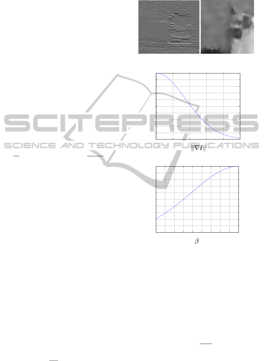
5.2 New Perceptual Diffusion Scheme
In (Alvarez et al., 1992), the aim is to restrict the
diffusion process only along the tangential direction
to the gradient and tuned by the gradient magnitude.
Here, we aim to diffuse only in the θ
1
and θ
2
direc-
tions in regions of pixels classified as edge points.
Firstly, we control the diffusion in function of the gra-
dient magnitude and secondly in function of the angle
between the two directions of the diffusion θ
1
and θ
2
.
Fig 8 (a) and (b) shows a diffused image without con-
trol function where edges are lost and blurred.
In order to control the diffusion in function of the
gradient magnitude, we use the following function u:
u(k∇Ik) = e
−
k∇Ik
k
2
, with k ∈ [0,1]. (5)
(a) Diffused image without
control function.
(b) Zoom in (a).
0 0.2 0.4 0.6 0.8 1
0
0.1
0.2
0.3
0.4
0.5
0.6
0.7
0.8
0.9
1
u
(c) Control function u.
0 20 40 60 80 100 120 140 160 180
0
0.1
0.2
0.3
0.4
0.5
0.6
0.7
0.8
0.9
1
v
(d) Control function v.
Figure 8: Diffused image without any control function
where blurring effect is too important and the two functions
u and v.
Using the anisotropic perceptual edge detector, we
are able to control the diffusion in function of the an-
gle between θ
1
and θ
2
(see eq. 3) called β. Indeed, at
the level of one pixel, the more β is close to 0, the less
the diffusion is important. On the contrary, more β is
close to 180 (in degrees), more the smoothing is im-
portant. The angular control function v can be defined
as follows:
v(β) = e
−
180−β
180·h
2
, (6)
with h ∈ [0,1] and β = θ
1
− θ
2
[180](in degrees).
VISAPP 2012 - International Conference on Computer Vision Theory and Applications
60
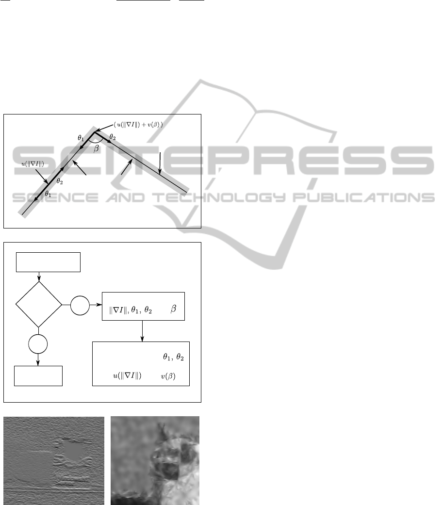
The new diffusion process presented in Fig. 9 (a)
and (b) is described by the following PDE :
∂I
t
∂t
= F
A
(I
0
)∆I
t
+(1− F
A
(I
0
))·
u(k∇Ik) + v(β)
2
∂
2
I
t
∂θ
1
∂θ
2
(7)
Contrary to (Alvarez et al., 1992), we do not want
to inhibit the diffusion at edges because the two direc-
tions of the diffusion θ
1
and θ
2
are sufficiently precise
to preserve contours. The values k = 0.5 and h = 0.8
enable to accurately control the diffusion along edges
and corners.
(Anisotropic diffusion)
Flat areas detected
Edge
Isotropic diffusion
/
Isotropic diffusion
(a) Schema of our diffusion.
Original image
Flat area
Computation of
Anisotropic diffusion
in function of
and
and
in two directions
( )
Isotropic
diffusion
detection
YES
NO
(b) Organigramm of our method.
(c) Diffused image, 15 itera-
tions.
(d) Zoom in (c).
Figure 9: Different steps of our diffusion scheme. (c)
and (d) correspond to the image in 7 (a) diffused with our
method, the blurring effect is small at edges.
6 EXPERIMENTAL RESULTS
In this section, we present some quantitative and qual-
itative results. In order to carry out some qualitative
results, we have conducted a number of tests with real
images. We analyzed the effect of adding a uniform
white noise on the original image using the following
formula:
I
m
= (1 −L) · I
0
+ L · I
N
with L ∈ [0,1],
where I
0
is the original image, I
N
an image of random
uniform noise, I
m
the resulting noisy image and L the
level of noise.
In our test, we performed an anisotropic diffusion
and compared our results with several methods.
6.1 Qualitative Results
We have called our approach PR for Perceptual image
Restoration. In the images presented in Fig. 11 (b)
and 12 (b), the aim is to smooth the noise present in
the different images preserving all objects. We used
our scheme with µ = 5, λ = 1 and ∆θ = 5
◦
for flat area
detection and the value of the threshold in amplitude
s
th
is equal to 0.05. Parameters used in anisotropic
edge detector in order to compute (θ
1
,θ
2
) are µ = 5,
λ = 1.5 and ∆θ = 2
◦
. The result of our anisotropic
diffusion is presented in the Fig. 11 (h), (i) and 12
(h), (i) after 5 or 10 iterations.
We compare our result with several approaches
as well as the well known Nagao (Nagao and Mat-
suyama, 1979) and bilateral filters (Tomasi and
Manduchi, 1998). We compare also with other
PDE’s approaches of Alvarez et al. (Alvarez et al.,
1992), Perona-Malik (Perona and Malik, 1990) and
Tschumperl
´
e (Tschumperl
´
e, 2006). For the bilateral
filter, Nagao filter and Perona-Malik method, results
are noisy in the different images (Fig. 11 and 12 (c),
(d), and (f)). The approaches of Alvarez et al. and
Tschumperl
´
e remove the noise but blur edges.
6.2 Influence of Noise
Curves have been plotted on Fig. 11 (j), (k) and 12
(j), (k), they present respectively the evolution of the
PSNR (Peak Signal to Noise Ratio) and RMSE. We
have compared our result after 5 and 10 iterations with
the bilateral filter, and the method of Tschumperl
´
e.
The bilateral filter is used with two iterations and the
algorithm of Tschumperl
´
e with 20 iterations and a
standard deviation of the gaussian σ = 1 for each test.
For low levels of noise (L < 0.5), our approach and
this of Tschumperl
´
e perform well in terms of this two
measures. After 10 iterations our result seems better
A NEW REGION-BASED PDE FOR PERCEPTUAL IMAGE RESTORATION
61
10 20 30 40 50 60 70 80 90
0
0.1
0.2
0.3
0.4
0.5
0.6
0.7
0.8
0.9
1
Noise level
SSIM
Man - SSIM
PR 5 iterations
PR 10 iterations
Bilateral filter
Tschumperlé
Noisy image
(a) Image in Fig. 11 (a).
10 20 30 40 50 60 70 80 90
0
0.1
0.2
0.3
0.4
0.5
0.6
0.7
0.8
0.9
1
Noise level
SSIM
House - SSIM
PR 5 iterations
PR 10 iterations
Bilateral filter
Tschumperlé
Noisy image
(b) Image in Fig. 12 (a).
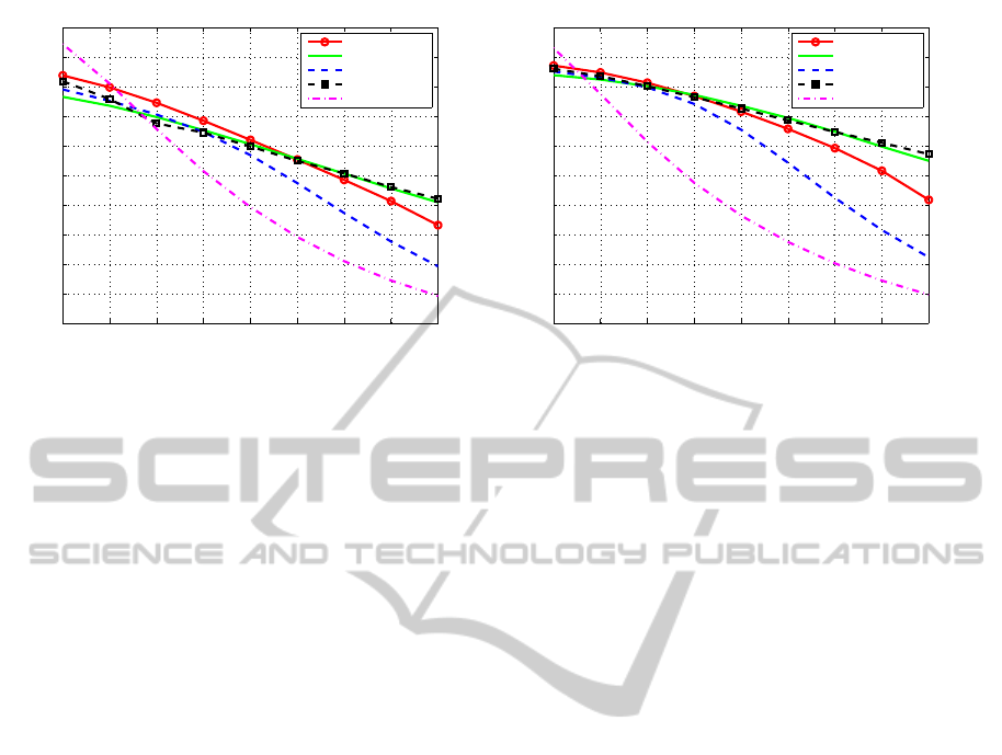
Figure 10: SSIM evolution in function of the noise level.
than 5 iterations when the noise is high. However,
PSNR and RMSE measures are not fully consistent
with human eye perception, that is why we have mea-
sured a similarity metric.
6.2.1 Perceptual Evolution
Instead of calculating a local difference like the PSNR
which does not take into account the perception of the
image, it exists a measure that estimates the similarity
between two images. This metric called SSIM (Struc-
tural SIMilarity) measures similar structures between
two images (Wang et al., 2004). It is based on several
windows of the image.
The measure will yield values between zero and
one, when the result is close to one, the structures are
considered as very well preserved. The total measure
of SSIM on the whole image is given by the average
SSIM on all windows.
Thus, we conducted SSIM measures plotted in
Fig. 10 in function of the level of noise on the two
images shown in Fig. 11 (a) and 12 (a). This measure
reflects better the preservation of the contours.
We observe, for our method, when the noise is less
than fifty percent in the image, compared to 10 iter-
ations, 5 iterations keeps the shape better but when
it exceeds this threshold, 10 iterations are necessary.
The difference in the SSIM decreases between 5 and
10 iterations for noise less than fifty percent when the
image is composed of fine textures on the image of
the house in Fig. 12 (a). Our approach removes the
fine textures and diffuse isotropically, resulting in a
loss of information compared to the original image.
Nevertheless, when the image is composed mainly
of small objects, the result of the SSIM seems better
for our approach with five iterations for the images
in Fig. 11 (a). On the contrary, an image composed
of large objects, like the house in Fig. 12 (a), SSIM
values crosses from a noise level of around forty per-
cent for 5 or 10 iterations. Beyond, 10 iterations are
necessary.
The bilateral filter gives good results when the
noise is small but the SSIM values decrease rapidly.
In general, Tschumperl
´
e’s scores are better than the
bilateral filter. However, our method with 10 itera-
tions gives the best results in terms of SSIM when the
noise level is between 30 and 70 percent (above 70
percent, the noise is too hard to compare such mea-
sures).
Fig. 13 shows a result of an ultrasound image of a
fetus composed of a high noise. After diffusion, edges
of the fetus are very sharped and the noise is totally
removed.
7 CONCLUSIONS
We have proposed in this paper a new method for dif-
fusing the noise in images by pixel classification us-
ing a rotating smoothing filter followed by a PDE.
Our classification method seems very promising as
we have been able to classify correctly homogenous
regions and edge regions for various image types. The
diffusion process that we have developed precisely
combines isotropic and anisotropic diffusion, and en-
ables to keep edges and corners of different objects
in highly noisy images. Comparing our results with
existing algorithms allows us to validate our method.
As introduced in Fig. 13, next on our agenda is to
enhance this method for medical images.
VISAPP 2012 - International Conference on Computer Vision Theory and Applications
62
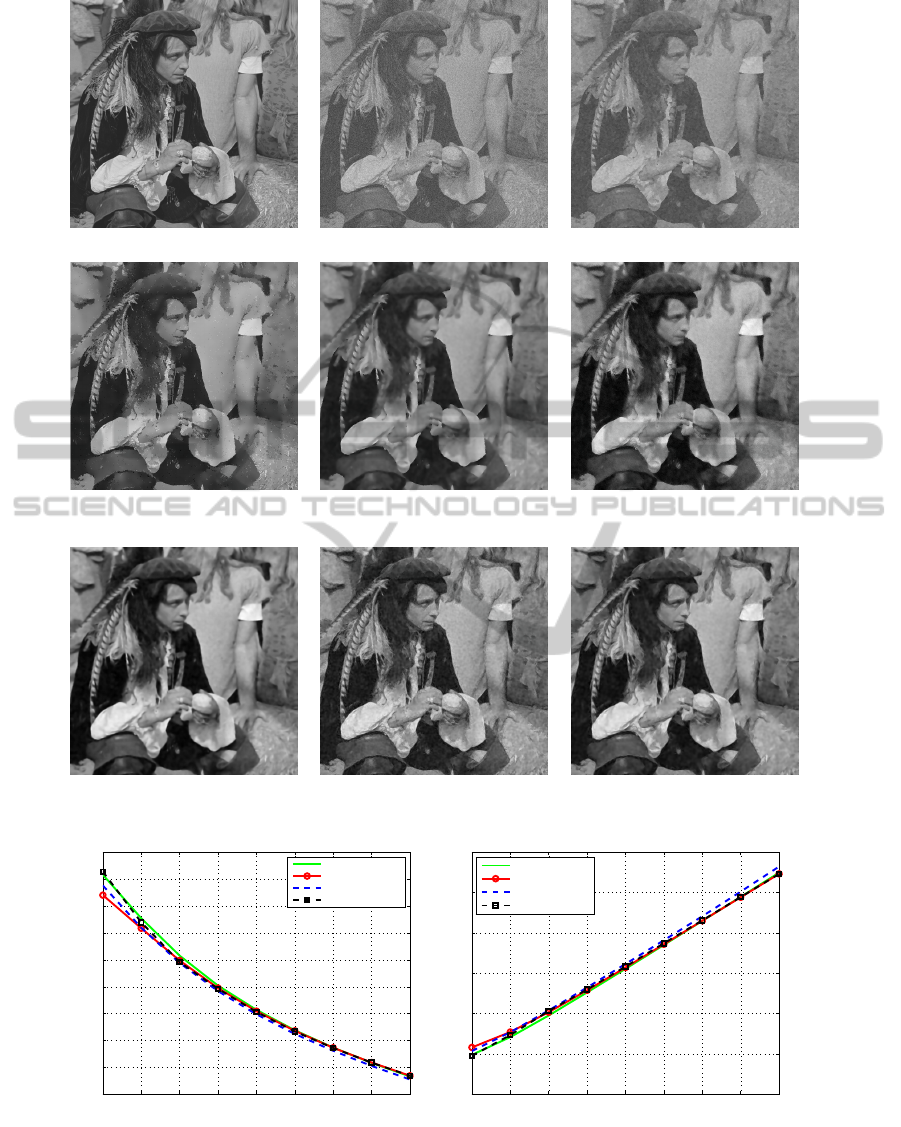
(a) Original image 256×256. (b) Noisy image, L = 0.7. (c) Nagao filter.
(d) Perona-Malik, (e) Alevarez et al. (f) Bilateral filter
100 iterations. 20 iterations. 2 iterations.
(g) Tschumperl
´
e, (h) Our algorithm (i) Our algorithm
20 iterations, σ=1. 5 iterations. 10 iterations.
0.1 0.2 0.3 0.4 0.5 0.6 0.7 0.8 0.9
12
14
16
18
20
22
24
26
28
30
Noise level
PSNR
PR 5 iterations
PR 10 iterations
Bilateral filter
Tschumperlé σ = 1
0.1 0.2 0.3 0.4 0.5 0.6 0.7 0.8 0.9
0
10
20
30
40
50
60
Noise level
RMSE
PR 5 iterations
PR 10 iterations
Bilateral filter
Tschumperlé σ = 1
(j) PSNR evolution. (k) RMSE evolution.
Figure 11: Image restoration on an image containing small objects.
A NEW REGION-BASED PDE FOR PERCEPTUAL IMAGE RESTORATION
63
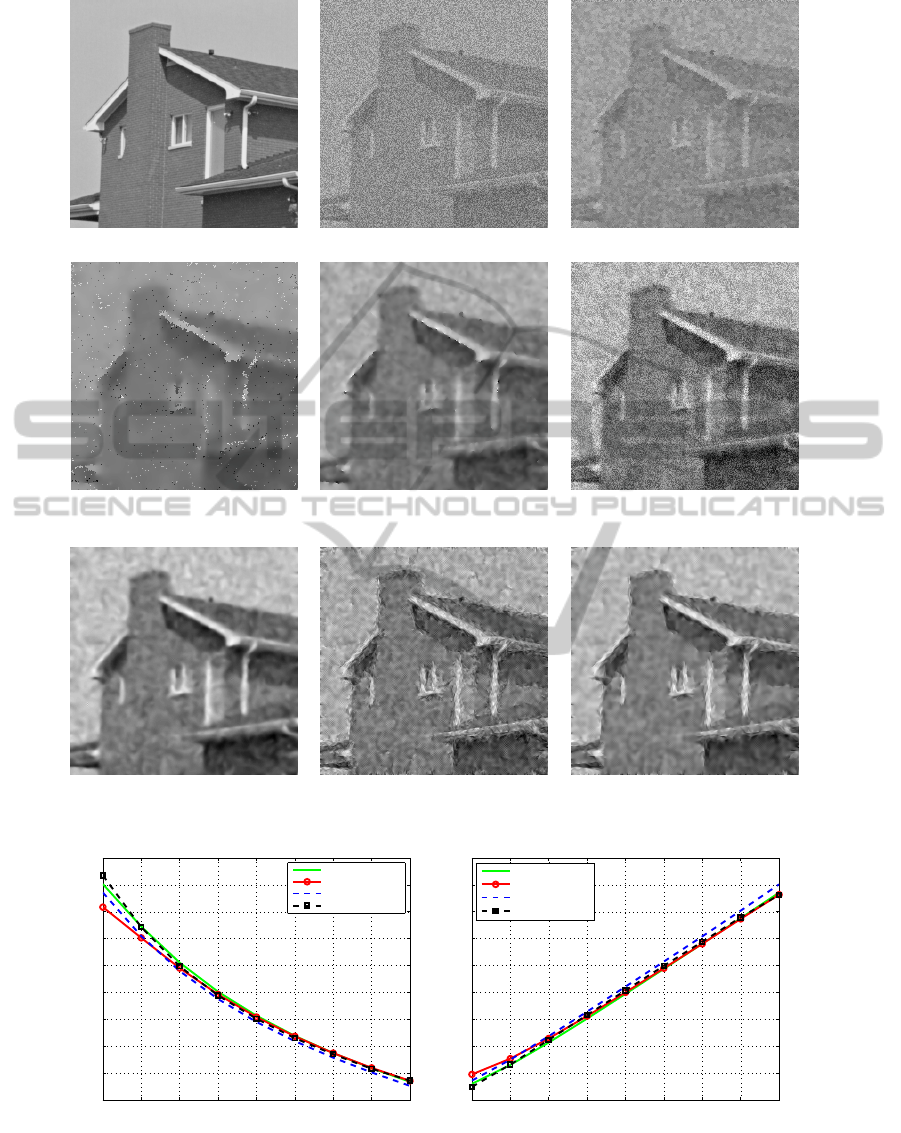
(a) Original image 256×256. (b) Noisy image, L = 0.7. (c) Nagao filter.
(d) Perona-Malik, (e) Alevarez et al. (f) Bilateral filter
100 iterations. 20 iterations. 2 iterations.
(g) Tschumperl
´
e, (h) Our algorithm (i) Our algorithm
20 iterations, σ=1 5 iterations. 10 iterations.
0.1 0.2 0.3 0.4 0.5 0.6 0.7 0.8 0.9
14
16
18
20
22
24
26
28
30
32
Noise level
PSNR
PR 5 iterations
PR 10 iterations
Bilateral filter
Tschumperlé σ = 1
0.1 0.2 0.3 0.4 0.5 0.6 0.7 0.8 0.9
5
10
15
20
25
30
35
40
45
50
Noise level
RMSE
BM 5 iterations
BM 10 iterations
Bilateral filter
Tschumperlé σ = 1
(j) PSNR evolution. (k) RMSE evolution.
Figure 12: Image restoration on an image containing large structures.
VISAPP 2012 - International Conference on Computer Vision Theory and Applications
64
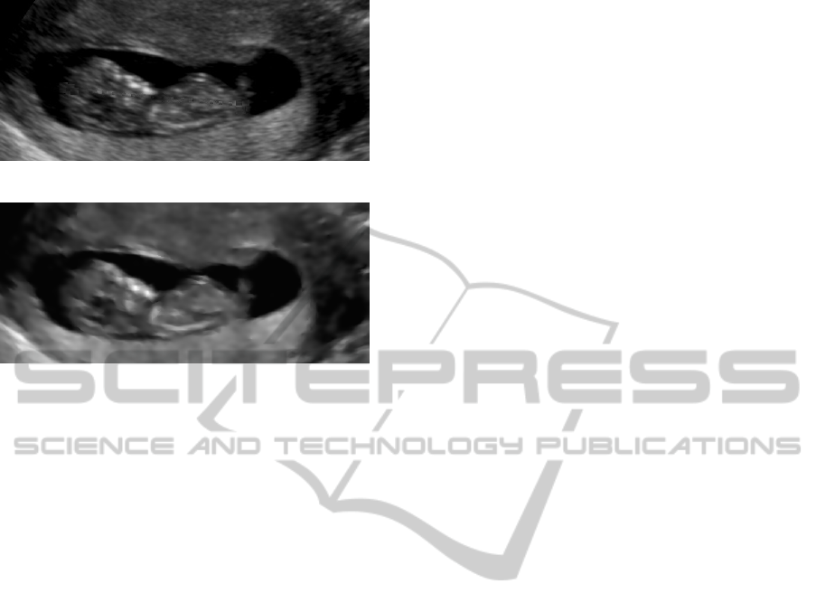
(a) Original image 533×231.
(b) Restored image.
Figure 13: Ultrasound image.
REFERENCES
Alvarez, L., Lions, P.-L., and Morel, J.-M. (1992). Image
selective smoothing and edge detection by nonlinear
diffusion, ii. SIAM Journal of Numerical Analysis,
29(3):845–866.
Aubert, G. and Kornprobst, P. (2006). Mathematical prob-
lems in image processing: partial differential equa-
tions and the calculus of variations (second edition),
volume 147. Springer-Verlag.
Black, M., Sapiro, G., Marimont, D., and Heeger, D.
(1998). Robust anisotropic diffusion. IEEE Trans-
actions on Image Processing, 7(3):421–432.
Catt
´
e, F., Dibos, F., and Koepfler, G. (1995). A morpholog-
ical scheme for mean curvature motion and applica-
tions to anisotropic diffusion and motion of level sets.
SIAM J. Numer. Anal., 32:1895–1909.
Deriche, R. (1992). Recursively implementing the gaussian
and its derivatives. In International Conference On
Image Processing. A longer version is INRIA Research
Report RR-1893, pages 263–267.
Freeman, W. T. and Adelson, E. H. (1991). The design and
use of steerable filters. IEEE Transactions on Pattern
Analysis and Machine Intelligence, 13:891–906.
Jacob, M. and Unser, M. (2004). Design of steerable filters
for feature detection using canny-like criteria. IEEE
Transactions on Pattern Analysis and Machine Intel-
ligence, 26(8):1007–1019.
Magnier, B., Montesinos, P., and Diep, D. (2011a). Fast
Anisotropic Edge Detection Using Gamma Correction
in Color Images. In IEEE 7th International Sympo-
sium on Image and Signal Processing and Analysis,
pages 212–217.
Magnier, B., Montesinos, P., and Diep, D. (2011b). Ridges
and valleys detection in images using difference of ro-
tating half smoothing filters. In Advances Concepts
for Intelligent Vision Systems, pages 261–272.
Magnier, B., Montesinos, P., and Diep, D. (2011c). Texture
Removal in Color Images by Anisotropic Diffusion.
In International Conference on Computer Vision The-
ory and Applications (VISAPP 2011), pages 40–50.
Montesinos, P. and Magnier, B. (2010). A New Perceptual
Edge Detector in Color Images. In Advances Concepts
for Intelligent Vision Systems, pages 209–220.
Nagao, M. and Matsuyama, T. (1979). Edge preserving
smoothing. CGIP, 9:394–407.
Perona, P. (1992). Steerable-scalable kernels for edge detec-
tion and junction analysis. IMAVIS, 10(10):663–672.
Perona, P. and Malik, J. (1990). Scale-space and edge
detection using anisotropic diffusion. IEEE Trans-
actions on Pattern Recognition and Machine Intelli-
gence, 12:629–639.
Tomasi, C. and Manduchi, R. (1998). Bilateral filtering for
gray and color images. In International Conference
on Computer Vision, pages 839–846. IEEE.
Tschumperl
´
e, D. (2006). Fast anisotropic smoothing
of multi-valued images using curvature-preserving
PDE’s. International Journal of Computer Vision,
68(1):65–82.
Tschumperl
´
e, D. and Deriche, R. (2005). Vector-valued im-
age regularization with pdes: A common framework
for different applications. IEEE Transactions on Pat-
tern Analysis and Machine Intelligence, pages 506–
517.
Wang, Z., Bovik, A., Sheikh, H., and Simoncelli, E. (2004).
Image quality assessment: From error visibility to
structural similarity. Image Processing, IEEE Trans-
actions on, 13(4):600–612.
Weickert, J. (1998). Anisotropic diffusion in image process-
ing. Teubner-Verlag, Stuttgart, Germany.
A NEW REGION-BASED PDE FOR PERCEPTUAL IMAGE RESTORATION
65
