MCMC PARTICLE FILTER WITH OVERRELAXATED SLICE
SAMPLING FOR ACCURATE RAIL INSPECTION
Marcos Nieto
1
, Andoni Cort´es
1
, Oihana Otaegui
1
and I˜nigo Etxabe
2
1
Vicomtech-IK4 Research Alliance, Donostia-San Sebasti´an, Spain
2
Datik, Donostia-San Sebasti´an, Spain
Keywords:
Computer Vision, Particle Filter, Slice Sampling, Laser, Rail Inspection.
Abstract:
This paper introduces a rail inspection system which detects rail flaws using computer vision algorithms.
Unlike other methods designed for the same purpose, we propose a method that automatically fits a 3D rail
model to the observations during regular services and normal traffic conditions. The proposed strategy is
based on a novel application of the slice sampling technique with overrelaxation in the framework of MCMC
(Markov Chain Monte Carlo) particle filters. This combination allows us to efficiently exploit the temporal
coherence of observations and to obtain more accurate estimates than with other techniques such as importance
sampling or Metropolis-Hastings. The results show that the system is able to efficient and robustly obtain
measurements of the wear of the rails, while we show as well that it is possible to introduce the slice sampling
technique into MCMC particle filters.
1 INTRODUCTION
Defect detection systems for rail infrastructure are ut-
terly needed to reduce train accident and associated
costs while increase transport safety. The early de-
tection of wear and deformation of tracks optimises
maintenance scheduling and reduces costs of periodic
human inspections. For that purpose it is required
the introduction of new technological developments
that make these systems more efficient, easier to in-
stall and cheaper for rail operators. Specifically, some
magnitudes are of vital importance, such as the wear
of the rails, and the widening of the track, which
may cause catastrophic derailment of vehicles (Can-
non et al., 2003).
Traditionally, this problem has been faced us-
ing human inspection, or tactile mechanical devices
which analyse the profile of the tracks while installed
in dedicated rail vehicles running at low speed. Cur-
rent technological trends try to avoid using contact-
based devices to avoid their practical problems. Some
works are based on the use of ultrasonic guided waves
(di Scalea et al., 2005), which allow the detection
of surface-breaking cracks and sizing of transverse;
and vision-based systems, that determine the presence
and magnitude of visible flaws (Alippi et al., 2000).
Due to the rail geometry, lasers are typically used to
project a line on the rail to ease the detection of its
profile.
Regarding vision systems applied in this field,
massive amounts of data are typically acquired and
stored for a supervised posterior analysis stage to ac-
tually identify and locate defects. A major lack in this
type of applications is the automatic fit of the model
of the rail to the detections so that the potential wear
of the rail could be automatically analyzed to see if it
falls within the tolerances. The challenge of a vision-
system in this field is to fit a planar 3D model of a rail
to a set of 2D observations of laser projections in the
abscence of reliable visual features that generate met-
ric patterns (a pair of points with known distance, or
a known angle between imaged lines). Some authors
(Alippi et al., 2000) (Alippi et al., 2002) have omitted
this problem and work at image level, which includes
the inherent projective distortion into their measure-
ments. Popular computer vision tools fail in this task,
such as POSIT (DeMenthon and Davis, 1995) since
it does not work for planar structures, or optimisa-
tion methods, such as gradient-descent of Levenberg-
Marquardt algorithm (Nocedal and Wright, 2006),
which are extremely sensitive to local minima.
In this paper we propose an automatic method
for rail auscultation using a vision-based system that
fits a 3D model of the rail to the observations us-
ing a MCMC (Markov Chain Monte Carlo) particle
filter. The method performs estimates of the proba-
164
Nieto M., Cortés A., Otaegui O. and Etxabe I..
MCMC PARTICLE FILTER WITH OVERRELAXATED SLICE SAMPLING FOR ACCURATE RAIL INSPECTION.
DOI: 10.5220/0003853901640172
In Proceedings of the International Conference on Computer Vision Theory and Applications (VISAPP-2012), pages 164-172
ISBN: 978-989-8565-04-4
Copyright
c
 2012 SCITEPRESS (Science and Technology Publications, Lda.)

90º
laser camera
90º
head
web
foot
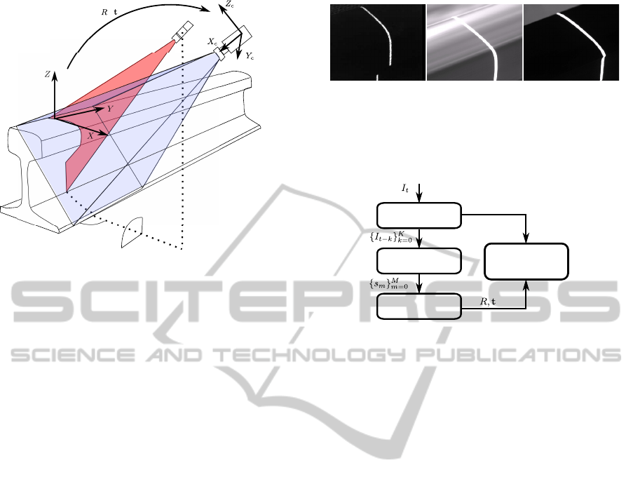
Figure 1: Set-up of the elements of the system. The laser
is installed orthogonal to the rail, while the camera shows
some rotation and translation {R, t}.
bility density function of the model through time by
applying the overrelaxation slice sampling technique,
which provides accurate and robust fits while reduc-
ing the number of required evaluations of the poste-
rior function compared to other schemes such as im-
portance sampling or Metropolis-Hastings.
This paper is organized as follows: section 2 illus-
trates the architecture of the method; in section 3 the
image processing techniques used for laser detection
are explained; section 4 shows in detail the proposed
particle filter strategy to fit the 3D model to the obser-
vations and section 5 depicts the procedure to project
the 2D image elements into 3D to retrieve the actual
metric error measurements. Tests and discussion are
presented in section 6.
2 SYSTEM DESCRIPTION
The system has been devised to measure two impor-
tant magnitudes: the wear of the rails, and the widen-
ing of the track. For that purpose, one camera and a
laser are installed for each rail, which are set-up as
depicted in figure 1. As shown, the only requirement
is that the laser line is orthogonally projected to the
rail, i.e. the laser plane coincides with Y = 0. The
camera monitorises the projected line with a certain
angle to acquire images as those shown in figure 2.
This angle can be any that guarantees that the laser
line is observed in its projection on both the head and
web of the rail.
It is noteworthy that the system does not require
an exact positioning or simmetry of the cameras with
respect to the rails, since the vision-based algorithm
(a) (b) (c)
Figure 2: Examples of images captured by the acquisition
system: (a) typical static image; (b) image captured during
regular service, with sun reflections; and (c) severe rail head
wear.
3D model fit
Measurement
& Monitorization
Laser detection
Buffer
Figure 3: Block diagram of the proposed method.
automatically determines the relative position and ro-
tation {R, t} of the cameras with respect to their cor-
responding rail.
Figure 3 shows a block diagram of the system.
The first stage comprises the proposed method for
laser line detection, which feeds the 3D modeling
stage that projects a specific rail model (for in-
stance we use the UIC-54 flat-bottom rail model) and
finds the best translation and rotation parameters that
makes the model fit to the observations. The last step
is the reprojection of the detected points given the es-
timate of the model parameters to quantitatively deter-
mine the wear of the rail and the existing widening.
3 LASER DETECTION
This section describes the proposed procedure to ex-
tract the information relative to the rail profile from
the images acquired by the system. In this harsh sce-
nario two main problems arise. On the one hand,
achieving a good isolation between the projection of
the laser line and other illuminated elements (e.g.
background elements reflecting the direct sun radia-
tion). On the other hand, obtaining time coherent in-
formation despite the relative movement that the rails
will show during regular services. The movement is
caused by vibrations, curvature (the width of the track
changes accordingly to the curve radius), or the rela-
tive position of the cameras with respect to the wheels
(the more distance to the wheel, the more movement
of the rail with respect to the bogie).
MCMC PARTICLE FILTER WITH OVERRELAXATED SLICE SAMPLING FOR ACCURATE RAIL INSPECTION
165

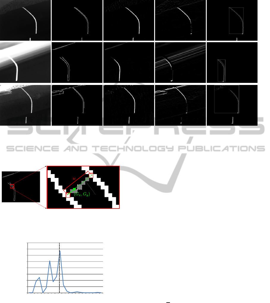
(a) (b) (c) (d) (e)
Figure 4: Examples of the proposed laser detection methodology for different cases (shown in rows): (a) original image; (b)
Canny edges; (c) G
x
, magnitude of gradient x-component; (d) G
y
, magnitude of gradient y-component; and (e) connected
component analysis.
Figure 5: Estimation of the width of the laser beam. The
middle point between the start and end points is used to
compute the mean intensity level of the laser line.
0
20
40
60
80
100
120
140
160
1 2 3 4 5 6 7 8 9 10 11 12 13 14 15 16 17 18 19 20 21 22
Count
Beam width
Ground truth
Figure 6: Histogram of width values for the example images
of figure 4 middle row.
The laser line can be described by its visual char-
acterizes. First, since we do use an infrarred filter,
the laser line is imaged as a bright stripe compared to
the rest of the image, which remains dark (save for
the reflective surfaces). Second, the laser line width
can be considered fixed independently of the position
in the image, since the relative distance between the
different points in the rail is too low and causes no
significant perspective effect.
According to these two considerations, the pro-
posed method carries out the following actions (which
are depicted with images in figure 4). First, we apply
the Canny edge detector, which identifies the edges of
the image, and we keep the gradient values (G
x
, G
y
)
it internally computes using the Sobel operator (Gon-
zalez and Woods, 2002). From each identified edge
pixel, we search in the gradient direction the closest
edge pixel and store the obtained distance as a mea-
sure of the width of the stripe (see figure 5). Since we
do have edges that do not belong to the laser stripe,
a histogram analysis is carried out to select the most
repeated distance value w
t
. An example histogram
is shown in figure 6, where the ground truth value is
shown with a dashed line. As shown, the detected
maximum of the histogram is very close to the ground
truth. This value is averaged in time to adapt the sys-
tem measurements to the observations, so that we ob-
tain ˆw
t,K
=
1
K
∑
K
k=1
ˆw
t− k
.
Since we do have an instantaneous estimate of
ˆw
t,K
at each time instant (except for the very first
frame), we can as well characterise the intensity level
of the laser line by analyzing the intensity level of the
middle pixels between pairs of edge points whose dis-
tance is close to ˆw
t,K
. With this analysis we obtain the
mean µ
I
and standard deviation σ
I
of the intensity val-
ues I(x, y) of the pixels likely belonging to the laser
stripe.
VISAPP 2012 - International Conference on Computer Vision Theory and Applications
166

From the information extracted at pixel-level, it is
possible to search for the laser stripes at a higher level.
The search is carried out locating pairs of edge points
that likely belong to the laser. A pair p
i
is defined as
a couple of points which define the left and right limit
of the projected laser line and whose distance is close
to ˆw
t,K
. To reduce the algorith complexity, we define
pairs at row level, i.e.
p
i
= {(x
l
, x
r
, y) \|x
r
−x
l
− ˆw
t− K
| < ε} (1)
where x
l
and x
r
are the x-coordinates of the points of
the pair, y is their common vertical coordinate; and ε
is an error limit that can be safely set as a percentage
of the width value, e.g. ε = 0.05 ˆw
t− K
.
The intensity level information is used to classify
pairs in connected groups so that the different parts
of the laser projection (the corresponding to the head
and the web of the rail) can be identified. This classi-
fication will allow having a better model fit. For that
purpose a thresholded image is created from I using
as threshold µ
t,K
−2σ
t,K
. For each pair we can de-
fine a label that identifies the connected component it
belongs to, c
i
= m.
Finally we obtain stripes as sets of pairs which be-
long to the same connected component of the inten-
sity binarized image: s
m
= {p
i
\c
i
= m}. From here
on we will denote a pair p
i
as p
m,i
where m identifies
the cluster or stripe s
m
it belongs to.
To reduce the impact of outliers those sets of pairs
whose cardinality is lower than 3 are removed, i.e.
there must be at least 3 connected pairs to define a
stripe. Two main stripes are finally identified amongst
the stripes. As shown in figure 4 (e) the lower vertical
stripe corresponds to the rail web, and the largest one
defines the head of the rail. The lower point of the
head stripe will be denoted as anchor point, and used
as a reference point to fit the 3D model.
4 3D MODEL FIT
To actually be capable of determining the existing
wear of the rail, it is necessary to fit the rail model
to the observations extracted from the images. The
observation of image I
t
is defined as z
t
= {s
m
}
M
m=1
,
i.e. a set of M stripes.
The model fit must be such that describes the rel-
ative movement between the rail and the camera, so
that we obtain a common coordinate system for the
model and the observation and measure the potential
defects.
From the projective geometry point of view, there
is an unsolved ambiguity in the projection of a 3D
planar model to a 2D observation with unkown scale:
a single 2D observation can be the projection of the
model at different positions and distances.
Therefore, the problem consists on finding the rel-
ative traslation and rotation between each camera with
its corresponding rail. This way, for each camera we
can define the state vector to be estimated at each time
instant t as x
t
= (x, y, z, θ, ˙x, ˙y, ˙z,
˙
θ)
⊤
, where (x, y, z) are
the translation components of each coordinate axis
and θ is the rotation in the y-axis (the rotation of the
other angles can be considered negligible). The last
four elements correspondto the first derivative of each
of the four former parameters. We will assume that
the intrinsic parameters of the camera are computed
at the set-up and installation stage so that the projec-
tion matrix is already computed and available.
In this work we propose to apply Bayesian infer-
ence concepts that allow us to propagate the proba-
bility density function of the state vector conditioned
to the knowledge of all observations up to time t,
p(x
t
|z
1:t
). Within this framework we will be able to
overcome the mentioned ambiguity and achieve accu-
rate estimates of the target coordinate systems so that
the rail defects can be measured.
4.1 MCMC Particle Filter
MCMC methods have been successfully applied to
different nature tracking problems (Khan et al., 2005;
Barder and Chateau, 2008). They can be used as a tool
to obtain maximum a posteriori (MAP) estimates pro-
vided likelihood and prior models. Basically, MCMC
methods define a Markov chain, {x
(s)
t
}
N
s
s=1
, over the
space of states, x, such that the stationary distribution
of the chain is equal to the target posterior distribu-
tion p(x
t
|z
1:t
). A MAP, or point-estimate, of the pos-
terior distribution can be then selected as any statis-
tic of the sample set (e.g. sample mean or robust
mean), or as the sample, x
(s)
t
, with highest p(x
(s)
t
|z
1:t
),
which will providethe MAP solution to the estimation
problem. Compared to other typical sampling strate-
gies, like sequential-sampling particle filters (Aru-
lampalam et al., 2002), MCMC directly sample from
the posterior distribution instead of the prior density,
which might be not a good approximation to the op-
timal importance density, and thus avoid convergence
problems.
If we hypothesize that the posterior can be ex-
pressed as a set of samples
p(x
t− 1
|Z
t− 1
) ≈
1
N
s
N
s
∑
s=1
δ(x
t− 1
−x
(s)
t− 1
) (2)
then
p(x
t
|Z
t− 1
) ≈
1
N
s
N
s
∑
s=1
p(x
t
|x
(s)
t− 1
) (3)
MCMC PARTICLE FILTER WITH OVERRELAXATED SLICE SAMPLING FOR ACCURATE RAIL INSPECTION
167

We can directly sample from the posterior distri-
bution since we have its approximate analytic expres-
sion (Khan et al., 2005):
p(x
t
|Z
t
) ∝ p(z
t
|x
t
)
N
s
∑
s=1
p(x
t
|x
(s)
t− 1
) (4)
For this purpose we need a sampling strategy, such
as the Metropolis-Hastings (MH) algorithm, which
dramatically improves the performance of traditional
particle filters based on importance sampling.
Nevertheless, there are other sampling strategies
that can be applied in this context and that improve
the performance of MH, reduce the dependency on
parameters and increase the accuracy of the estima-
tion using the same number of evaluations of the tar-
get posterior. Next subsection introduces the slice
sampling algorihtm, that was designed to remove the
problem of random walk detected in MH (Neal, 1998;
Neal, 2003).
4.2 Markov Chain Generation
Particle filters infer a point-estimate as an statistic
(typically, the mean) of a set of samples. Conse-
quently, the posterior distribution has to be evaluated
at least once per sample. For high-dimensional prob-
lems as ours, MCMC-based methods typically require
the use of thousands of samples to reach a stationary
distribution. This drawback is compounded for im-
portance sampling methods, since the number of re-
quired samples increases exponentially with the prob-
lem dimension.
In this work we propose to use the overrelaxated
slice sampling strategy (Neal, 1998), which avoids
random walks in the generation of the Markov Chains
and thus allows obtaining better descriptions of the
posterior distribution.
4.2.1 Slice Sampling
This technique generates a chain of samples, {x
k
}
N
k=1
from a arbitrary target pdf, p(z) (Neal, 2003). The
only requirement to apply this algorithm is that the
value p(x) can be evaluated for any given value of
x. As described by (Bishop, 2006), the slice sam-
pling improves the results, in terms of efficiency, of
typical sampling approaches based on the Metropolis-
Hastings (MH) algorithm (Gilks et al., 1996). MH has
an important drawback that makesit inefficient for the
proposed application as it is sensible to the step size,
given by the proposal distribution. If it is chosen too
small, the process behave as a random walk, which
makes the algorithm converge very slowly and, on the
contrary, if it is too large, the rejection rate may be
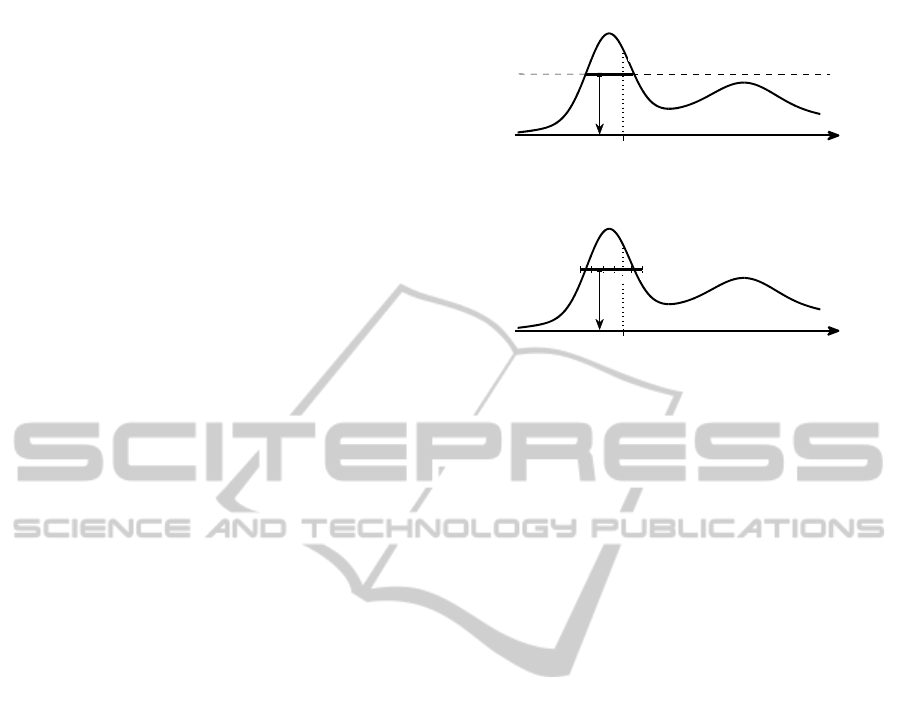
p(x
k − 1
)
x
k − 1
x
k
x
u
(a)
p(x
k − 1
)
x
k
x
k − 1
x
u
x
1
x
0
(b)
Figure 7: Univariate slice sampling: (a) the uniform u value
determines the slice through p(x); and (b) the practical im-
plementation uses fixed length steps to determine the range
in which x is uniformly sampled.
very high, hence not achieving accurate results. The
advantage of the slice sampler is due to its ability to
automatically adapt its step size according to the char-
acteristics of the probability density function.
For a better understanding of the slice sampler,
let us consider first the univariate case. Slice sam-
pling works by augmenting x with an auxiliary ran-
dom variable u and then sample from the joint (x, u)
space. Given the previous sample x
k−1
, u is uniformly
drawn in the range [0, p(x
k−1
)]. Fixed u, the sample
x
k−1
is obtained from the “slice” through the distri-
bution defined by { x : p(x) > u}. This criterion
is illustrated in figure 7 (a). Nevertheless, it is dif-
ficult to find the limits of the slice and thus to draw
a sample from it. For that reason an approximation
is done by means of creating a quantized local slice,
delimited by x
0
and x
1
as shown in figure 7 (b). To
obtain these limits, the value p(x) is evaluated at left
and right of x
k−1
using fixed length steps (the quan-
tification step) until p(x) < u. The next sample, x
k
, is
obtained by uniformly sampling on this range (itera-
tively until p(x
k
) > u).
For multidimensional problems, the one-
dimensional strategy can be applied repeatedly on
every single dimension to obtain the samples.
4.2.2 Overrelaxated Slice Sampling
The overrelaxation method consists on the automatic
generation of a new sample given the defined slice
without the need of using a uniform random sample
between the slice limits. When the slice is defined,
the next sample value x
t− 1
is defined as the symmetric
point between the middle of the slice limits and the
VISAPP 2012 - International Conference on Computer Vision Theory and Applications
168

start point x
k−1
.
This simple step reduces the rejection rate of sam-
ples in many situations, since the probability of the
symetric point x
t− 1
to have a function value lower
than u is very reduced (it only will occur if the pre-
vious point was actually in the limit of the slice).
4.3 Likelihood Function
The likelihood function determines the evaluation of
each sample of the chain x
(s)
t
with respect to the ob-
servation at each time instant. Formally, this function
determines the probability of observing z
t
given a cer-
tain state vector hypothesis x
(s)
t
.
In our case, the observations correspond to the
detected laser stripes, while each sample x
(s)
t
deter-
mines a hypothesized position and rotation of the 3D
model. With the camera calibration information we
can project this model to the image and define a cost
function that determines how good the projected mod-
els fit to the detected stripes.
The model can be defined as a ser of coplanar
control points {c
i
= (X
i
, 0, Z
i
)}
N
i=1
in Y = 0. Writ-
ten in homogeneous coordinates we have {X
i
=
(X
i
, 0, Z
i
, 1)
⊤
}
N
i=1
. For each sample proposed by the
particle fitler, we do have a traslation and rotation of
the model which is applied to each control point:
X
(s)
i
= R
(s)
X
i
+ C
(s)
(5)
The result is projected into the image plane using
the camera projection matrix: x
(s)
i
= PX
(s)
i
.
The likelihood function can be defined as the
weighted sum of two functions. One of them re-
lated to the distance between the anchor point of the
projected model and the observed strokes, p(z
t
, x
(s)
t,a
).
The anchor point is the point that separates the head
and the web of the rail. The second term is related to
the goodness of fit of the rest of the model, p(z
t
, x
(s)
t,b
):
p(z
t
|x
(s)
t
) = αp(z
t
, x
(s)
t,a
) + (1−α)p(z
t
|x
(s)
t,b
) (6)
The first term, related to the anchor point is de-
fined as a normal distribution on the distance between
the observed and reference point:
p(z
t
|x
(s)
t,a
) =
1
√
2πσ
a
exp −
1
2
d
2
(x
(s)
t,a
, z
t,a
)
σ
2
a
!
(7)
where z
t,a
is the 2D position of the anchor point and
σ
a
is the standard deviation that characterizes the ex-
pected observation noise of the anchor point.
For the second term we first loop over the pro-
jected model points and search for the closest left and
right points of a pair p
i
. In case there is no pair closer
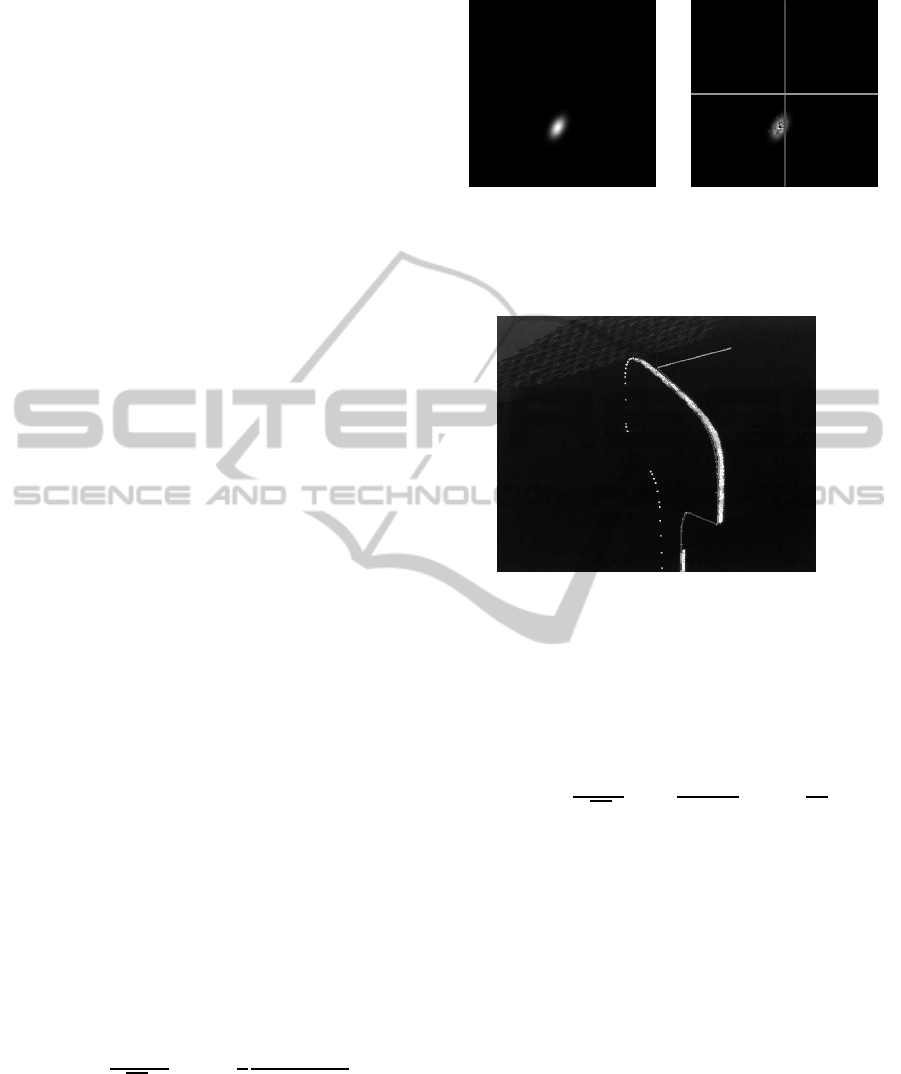
(a) (b)
Figure 8: Visualization of the likelihood map of the (x, y)
dimension: (a) likelihood map; (b) likelihood map and the
set of samples obtained with the slice sampling strategy.
Figure 9: An example hypothesis drawn by the sampler.
than a defined threshold, no points are associated with
that model point. When the points are found, the
counters N
l
and N
r
are increased, and the distance be-
tween the model point and the left and right points are
accumulated as d
l
and d
r
.
The second term can be then described as:
p(z
t
|x
(s)
t,b
) =
1
√
2πσ
∑
i={l,r}
N
i
2N
model
exp

−
d
2
i
σ
2

(8)
where N
model
is the number of model points. Since
this function uses both left and right fitting, it gives
high likelihood values for models that project be-
tween the left and right edges of the laser beam, which
enhances the accuracy of the fit compared to using
only one of the edges.
For a better visualization, we have computed the
likelihood value of all the possible valuesof the model
state vector spanning its x and y-coordinates for an ex-
ample image. The result can be seen in figure 8 where
the likelihood map is depicted as an intensity image,
where the brighter pixels correspond to (x, y) posi-
tions with higher likelihood value, and darker ones
with lower value. As shown, the likelihood function
is a peaked and descending function that can be easily
sampled with the proposed slice sampling procedure.
In figure 8 (b) we can see as well the obtained sam-
ples, which actually fall in the regions of the space
MCMC PARTICLE FILTER WITH OVERRELAXATED SLICE SAMPLING FOR ACCURATE RAIL INSPECTION
169

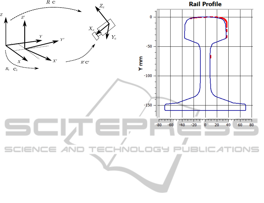
Figure 10: Relationship between the initial coordinate sys-
tem {X,Y, Z}, the camera coodinate system, {X
c
,Y
c
, Z
c
}
and the coordinate system defined after the application of
the correction provided by the particle filter {X
′
,Y
′
, Z
′
}.
with higher likelihood values. In figure 9 an exam-
ple model fit is depicted. The color code of the axes
of the coordinate frame helps to understand the likeli-
hood map of figure 8.
5 RAIL WEAR AND WIDENING
When the model fit has been obtained, we know the
new coordinate system {X
′
,Y
′
, Z
′
} that best fit to the
observations, and that can be different from the initial
coordinate system {X,Y, Z} according to the potential
relative movements of the rail with respect to the cam-
era (typically when the train is in a curve). Figure 10
illustrates the different coordinate systems involved.
To analyze the observed profile and compare it
with the reference profile it is necessary to transform
back the observations from the 3D plane defined by
Y
′
= 0. We can do that by obtaining the new ex-
trinsic parameters of the camera coordinate system,
{R
′
, C
′
}, recompute the projection matrix P
′
that links
3D points in {X
′
,Y
′
, Z
′
} to points in the image and
reduce it to a 3 ×3 homography that defines the cor-
respondence between points in the image plane and
points in the Y
′
= 0.
The new extrinsic parameters can be computed
using the initial extrinsic parameters and the values
given by the filter as C
′
= R
−1
t
(C−C
t
) and R
′
= RR
t
.
The corrected projection matrix is defined as a
3 ×4 matrix P
′
= K[R
′
|−R
′
C
′
] that links 3D points
in homogeneous coordinates into image points as
x = P
′
X
′
. Given that the laser is projected onto plane
Y
′
= 0, we can reduce P
′
to a 3×3 homography H
′
as:
x = P
′



X
0
Z
1



= H
′


X
Z
1


(9)
Figure 11: Comparison of the reference UIC-54 model and
the backprojected laser points.
where H
′
= (p
1
, p
3
, p
4
) and p
i
is the i-th column of
P
′
.
The homography can be used to backproject the
laser points detected in the image into a rectified view
of planeY
′
= 0 where metric measurements of the rail
wear can be generated as shown in figure 11.
Finally, the widening of the track can be as well
computed as the X component of the relative trasla-
tion between the coordinate system {X
′
,Y
′
, Z
′
} of the
left camera and the right camera.
6 TESTS AND DISCUSSION
We have evaluated the performance of the proposed
strategy applying different sampling methods but us-
ing for them all the proposed likelihood function: se-
quential importance resampling (SIR) (Arulampalam
et al., 2002), Metropolis-Hastings (MH) (Bishop,
2006), Slice Sampling (Neal, 2003) and Overrelax-
ated Slice Sampling (OSS) (Neal, 1998).
Due to the dimensionality of the problem (6 DoF),
the SIR particle filter requires too many samples to
keep a low error fit. It has been shown that the num-
ber of samples SIR requires to that end grows expo-
nentially with the dimensionality of the problem. In
our case we have observed that SIR does not provide
stable results using the proposed likelihood function
for a reasonable number of particles (up to 10
4
).
We have implemented three MCMC sampling
methods that create Markov Chain, which are known
to be the solution to the dimensionality problem of
VISAPP 2012 - International Conference on Computer Vision Theory and Applications
170

Table 1: Eficiency comparison between slice sampling (SS) and overrelaxated slice-sampling (OSS).
Step = 1 (mm) SS OSS
Num. Samp. Num. Evals. Error(mm) Num. Evals. Error(mm) ∆Evals(%) ∆Error(%)
10 287 3.364 266 3.213 7.32 4.49
15 430 2.732 419 2.572 2.56 5.86
25 695 1.198 650 1.363 6.47 -13.77
50 1345 1.345 1221 1.635 9.22 -21.56
100 2977 1.057 2869 1.101 3.63 4.16
Step = 2 (mm) SS OSS
Num. Samp. Num. Evals. Error(mm) Num. Evals. Error(mm) ∆Evals(%) ∆Error(%)
10 249 3.454 283 3.553 -13.65 -2.87
15 354 2.235 313 2.322 11.58 -3.89
25 632 1.332 561 1.554 11.23 -16.67
50 1229 1.112 1095 1.223 10.90 -9.98
100 2477 0.988 2171 1.212 12.35 -22.67
Step = 4 (mm) SS OSS
Num. Samp. Num. Evals. Error(mm) Num. Evals. Error(mm) ∆Evals(%) ∆Error(%)
10 195 5.391 166 5.489 14.87 -1.82
15 395 3.325 312 2.665 21.01 19.85
25 602 2.156 481 1.559 20.10 27.69
50 1124 1.285 901 1.082 19.84 15.80
100 2229 0.998 1844 1.001 17.27 -0.30
SIR: MH, SS and OSS. The MH, as explained in
(Bishop, 2006)(Neal, 2003), suffers from the problem
of the selection of the proposal function. If a gaus-
sian function is used, the problem is to find the ad-
equate standard deviation for that proposal. We have
observed that we have a trade-offproblem: on the one
hand we need small deviations (less than 0.5 mm) to
appropriately model the posterior function, while MH
requires high values to move quickly in the state space
and avoid the random-walk problem. This trade-off is
not solved satisfactorily by the MH for the proposed
problem.
On the contrary, slice sampling is capable of find-
ing this trade-off, since its sampling methodology re-
lies on finding slices which guarantees a good adap-
tation to the posterior function shape. This capability
allows obtaining very accurate results, specially when
using small values for the steps that defines the slice.
The only problem of using small steps is that the def-
inition of the slice requires often a significant number
of evaluations of the posterior, which in turn reduces
the performance of the system. This drawback can
be partially solved using the overrelaxated slice sam-
pling, which reduces the number of evaluations to be
carried out.
We have carried out a test to compare the perfor-
mance of the system using the SS and the OSS meth-
ods. The test is run to fit the UIC-54 model on a
sequence with movement, to evaluate how good the
sampling alternatives fit when the posterior function
is changing from one frame to the next one. The com-
parison is based on the computation of the fit error.
The results are shown in table 1. As can be observed,
we have run the tests for different step values (1, 2
and 4 mm), and for different number of effective sam-
ples to be drawn by the sampling methods. The ta-
bles shows the number of evaluations required by the
methods to obtain such number of effective samples,
and the fit error, which is computed as the average
distance of the detected laser points reprojected into
plane Y
′
= 0. The last two columns show the relative
difference between these parameters for the SS and
the OSS.
As we can see, for small steps both methods per-
form similarly, requiring the OSS between 2 and 9%
less evaluations. Nevertheless, for larger steps, such
as for 2 mm and specially for 4 mm, the OSS shows
its best performance. With step equal to 4 mm, and
100 samples, OSS evaluates the posterior 1844 times,
while SS needs 2229, both of them obtaining almost
the same error fit. These results show that the OSS
is capable of more efficiently representing a probabil-
ity density function using the slice method, which al-
lows faster computation without sacrifying accuracy,
which remains close to 1 mm average fit error.
6.1 Future Work
This paper summarizes the achievementsreached dur-
ing the development of a system for the automatic in-
MCMC PARTICLE FILTER WITH OVERRELAXATED SLICE SAMPLING FOR ACCURATE RAIL INSPECTION
171

spection of rail wear and widening. At the time of
submitting this paper the project is in a development
stage, so that the results have been obtaining with a
preliminar prototype system. In the further stages of
the project, several improvements are planned and a
more detailed evaluation analysis which will integrate
localisation data to the detection of rail defects.
7 CONCLUSIONS
In this paper we have introduced a new methodology
for the early detection of rail wear and track widening
based on projective geometry concepts and a proba-
bilistic inference framework. Our approach presents
a scenario where its usage in regular services is possi-
ble, with low cost acquisition and processing equip-
ment, which is a competitive advantage over other
manual or contact methodologies. For that purpose,
we propose the use of powerful probabilistic infer-
ence tools that allow us to obtain 3D information
of the magnitudes to be measured from uncomplete
and ambiguous information. In this proposal we use
the overrelaxatedslice sampling technique, which im-
plies a step forward in MCMC methods due to its
reliability, versatility and greater computational effi-
ciency compared to other methods of the literature
that build Markov Chains.
ACKNOWLEDGEMENTS
This work has been partially supported by the Diputa-
cion Foral de Gipuzkoa under project RAILVISION.
REFERENCES
Alippi, C., Casagrande, E., Fumagalli, M., Scotti, F., Piuri,
V., and Valsecchi, L. (2002). An embedded system
methodology for real-time analysis of railways track
profile. In IEEE Technology Conference on Instru-
mentation and Measurement, pages 747–751.
Alippi, C., Casagrande, E., Scotti, F., and Piuri, V. (2000).
Composite real-time image processing for railways
track profile measurement. IEEE Transactions on In-
strumentation and Measurement, 49(3):559–564.
Arulampalam, M. S., Maskell, S., Gordon, N., and Clapp,
T. (2002). A tutorial on particle filters for on-
line nonlinear/non-gaussian bayesian tracking. IEEE
Transactions on Signal Processing, 50(2):174–188.
Barder, F. and Chateau, T. (2008). MCMC particle filter
for real-time visual tracking of vehicles. In IEEE In-
ternational Conference on Intelligent Transportation
Systems, pages 539–544.
Bishop, C. M. (2006). Pattern Recognition and Ma-
chine Learning (Information Science and Statistics).
Springer.
Cannon, D., Edel, K.-O., Grassie, S., and Sawley, K.
(2003). Rail defects: an overview. Fatigue & Fracture
of Engineering Materials & Structures, 26(10):865–
886.
DeMenthon, D. and Davis, L. S. (1995). Model-based ob-
ject pose in 25 lines of code. International Journal of
Computer Vision, pages 123–141.
di Scalea, F. L., Rizzo, P., Coccia, S., Bartoli, I., Fateh, M.,
Viola, E., and Pascale, G. (2005). Non-contact ul-
trasonic inspection of rails and signal processing for
automatic defect detection and classification. Insight
- Non-Destructive Testing and Condition Monitoring,
47(6):346–353.
Gilks, W., Richardson, S., and Spiegelhalter, D. (1996).
Markov Chain Monte Carlo Methods in Practice.
Chapman and Hall/CRC.
Gonzalez, R. and Woods, R. (2002). Digital Image Process-
ing. Prentice Hall.
Khan, Z., Balch, T., and Dellaert, F. (2005). MCMC-based
particle filtering for tracking a variable number of in-
teracting targets. IEEE Transactions on Pattern Anal-
ysis and Machine Intelligence, 27(11):1805–1819.
Neal, R. M. (1998). Suppressing random walks in
markov chain monte carlo using ordered overrelax-
ation. Learning in Graphical Models, pages 205–228.
Neal, R. M. (2003). Slice sampling. Annals of Statistics,
31:705–767.
Nocedal, J. and Wright, S. J. (2006). Numerical Optimiza-
tion. Springer.
VISAPP 2012 - International Conference on Computer Vision Theory and Applications
172